Second Order Optimization Methods

19 August 2020 - 21 mins read time
Tags: Calculus Linear Algebra Python

DISCLAIMER: The content here is something I’ve learnt recently, and not in much depth. It is possible some of it is inaccurate or insufficient to make complete sense. As I learn more, I will keep updating this article. Meanwhile, please let me know about any existing flaws.

In the previous post, I discussed iterative methods for estimating the optimum of a loss function. While this method is intuitive and converges well most of the time, it’s not the most stable of training algorithms. It has been seen that using second order derivative information of the loss functions can help reach convergence much faster, under some conditions. In this short post, I’ll discuss two such methods: Newton’s method, the Levenberg-Marquardt method and the BFGS method. But first, here’s some intuition on why second order derivative information is useful.

Why second order derivatives?

Recall the plot of our over-simplified loss function from earlier (if you’re new, just look at the plot below instead). Especially, I want to focus on the two parts of the function which I’ve marked as $A$ and $B$.

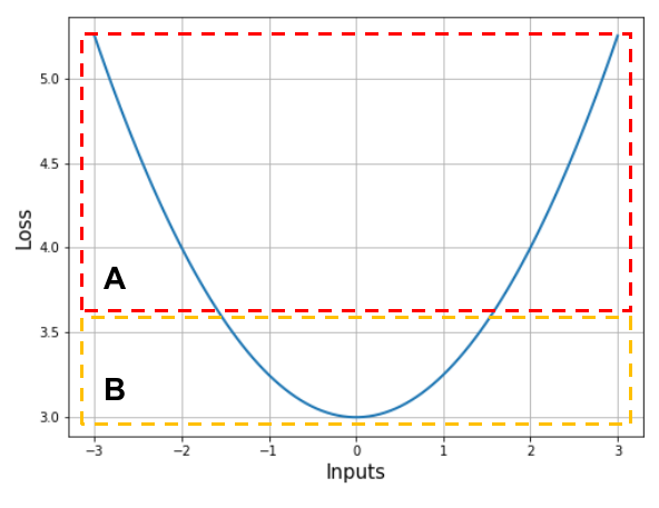
In section $A$, the slopes at points $1$ and $2$ are nearly the same; the loss function itself is nearly a straight line in that part. On the other hand, in section $B$, the slopes at points $1$ and $2$ have considerable difference.

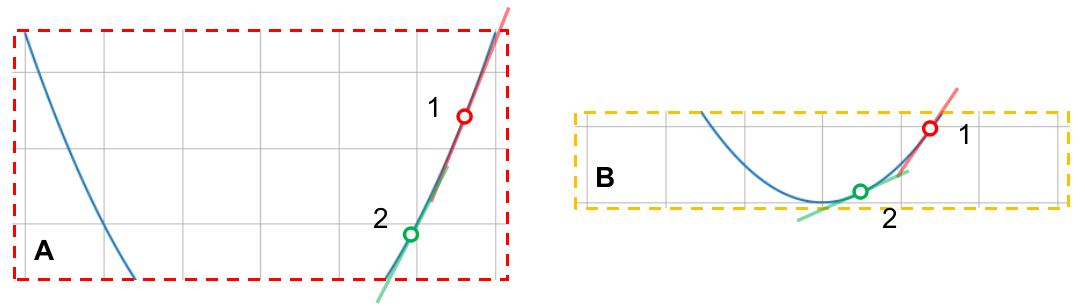
That being said, note that the points in section $A$ are further away from the minimum than those in section $B$. What does this tell us? When we are close to the minimum, the rate at which the slope of the loss function changes is higher than when we are far from it. Since the rate at which the loss function changes is its first order derivative (i.e. slope), the rate at which the slope itself changes is its second order derivative, which is sometimes referred to as its curvature. In section $A$, we have a low curvature region and in $B$, we have a high curvature region.

This is how second order derivatives can provide us unseful information about the loss function’s extrema. Let’s see how Newton’s Method exploits this phenomenon.

Newton’s Method

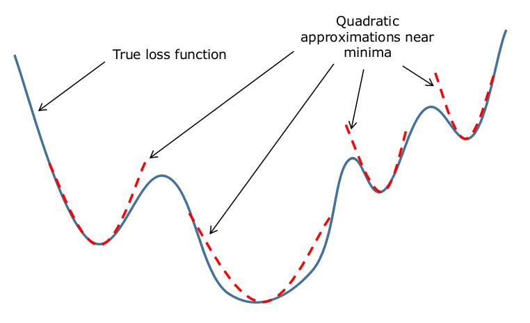
This method works on the fact that most loss functions can be approximated as quadratic functions when we are close to their minima. In a way, the over-simplified loss function we saw above is approximately how any loss function would look if we zoomed in on their minima.

That being said, we need some way to approximate the loss function at that point with a quadratic function. For this, we use the Taylor series approximation. In general, a scalar function $f(x)$ (a function whose inputs are scalar) can be approximated around a point $x_{0}$ in it’s domain with the following expression:

If $x$ is a vector instead of a scalar, then the equation modifies to the one shown below.

The accuracy of the approximation increases with inclusion of more terms in general. However, since we are dealing with vectors and we only want a second degree approximation, we will limit ourselves to the three terms shown in the second equation shown above. I’ve rewritten it below in simpler notation.

Just to be clear, our goal is to find some $\textbf{x}^{\ast}$ that minimizes our loss function. Like before, the derivative of the loss function at (the supposed minimizer) $\textbf{x}^{\ast}$ will be $0$. Before we perform the next step, there are some things I wish to state so that people unfamiliar with vector calculus may follow without much difficulty.

1. The second derivative of a function with respect to a vector is a matrix, often called the Hessian matrix of that function. For the vector $\textbf{x}$ shown below, the Hessian of $f(\textbf{x})$ will look like the one shown adjacent.

1. If $\textbf{a}$ and $\textbf{b}$ are vectors and $\textbf{M}$ is a matrix, each of compatible dimensions, then the following equations hold true.

If we differentiate the Taylor approximation with respect to $\textbf{x}$ and substitute $\nabla_{\textbf{x}}f(\textbf{x}^{\ast})=0$, we get the following equation.

I don’t see iterations here

We used the fact that $\nabla f(\textbf{x}^{\ast})=0$ at the minimum to solve for $\textbf{x}^{\ast}$ above. If that’s the case, shouldn’t $\textbf{x}^{\ast}$ be the minimizer we are looking for? Not quite, because the loss function $f(x)$ used up there is not the actual loss function but an approximation of it using the Taylor series. This approximation holds well in the neighborhood of $x_{0}$, and we have no reason to believe that $x_{0}$ falls at a location where the quadratic approximation holds good (if we knew the right place for $\textbf{x}_{0}$, we might as well have found the minimizer itself). Thus, we iteratively (and slowly) move in the direction suggested by the algorithm, hoping that we’ll land in the correct location in a while. In general, when sufficiently close to a minima, this method convergences faster than gradient descent. In general, the iterative update is represented with the equation below.

Example

Let’s have this working on some data. Since we do not have any auto-differentiation mechanism, we’ll have to provide the equations with the expressions for the Hessian and the gradients of the loss function. Our data is bivariate (has two independent variables), so $\textbf{H}$ will be a $(3\times 3)$ matrix (2 weights and a bias) and the vector of gradients will have size $(3\times 1)$. Also, remember that we are trying to tune $\Theta$, not $\textbf{x}$. To compute the quantities we want, we can write the loss function vectorially as shown and perform differentiation.

First, let’s make some imports and generate some data with the same parameters we used in the previous post.

import numpy as np 
import matplotlib.pyplot as plt

# Number of examples
N = 100

x_1 = np.random.normal(5, 1, size=N)
x_2 = np.random.normal(2, 1, size=N)
y = (5*x_1 + 2*x_2 + 5) + np.random.normal(0, 1, size=N)

Now let’s create the data matrix and initialize the parameters close to the actual values (zeros in this case). With a learning rate of 0.5, we’ll perform 20 parameter updates according to the rule above.

# Pad [x_1, x_2] with ones to create Z
Z = np.vstack((np.ones(N), x_1, x_2))

# Initialize params close to minimum
params = np.zeros((3, 1))

# Perform 20 update steps with learning rate 0.5
iterations = 20
eta = 0.5

for i in range(iterations):
    # Gradients vector
    grad = - Z.dot((y - params.T.dot(Z)).T)
    # Hessian matrix
    hess = - Z.dot(Z.T)
    # Perform parameter update
    params += eta * np.linalg.inv(hess).dot(grad)
    
    # Compute loss value and print
    loss = (0.5/N) * (y - params.T.dot(Z)).dot((y - params.T.dot(Z)).T)
    print("Iteration {:2d} - MSE Loss {:.4f}".format(i+1, loss[0][0]))
    
# Print final values of parameters
print("\nFinal parameter values:")
print("-----------------------------------------")
print("theta_1: {:.4f}".format(params[1][0]))
print("theta_2: {:.4f}".format(params[2][0]))
print("bias: {:.4f}".format(params[0][0]))

>>> Iteration  1 - MSE Loss 154.0395
    Iteration  2 - MSE Loss 38.8944
    Iteration  3 - MSE Loss 10.1082
    Iteration  4 - MSE Loss 2.9116
    Iteration  5 - MSE Loss 1.1125
    Iteration  6 - MSE Loss 0.6627
    Iteration  7 - MSE Loss 0.5502
    Iteration  8 - MSE Loss 0.5221
    Iteration  9 - MSE Loss 0.5151
    Iteration 10 - MSE Loss 0.5133
    Iteration 11 - MSE Loss 0.5129
    Iteration 12 - MSE Loss 0.5128
    Iteration 13 - MSE Loss 0.5127
    Iteration 14 - MSE Loss 0.5127
    Iteration 15 - MSE Loss 0.5127
    Iteration 16 - MSE Loss 0.5127
    Iteration 17 - MSE Loss 0.5127
    Iteration 18 - MSE Loss 0.5127
    Iteration 19 - MSE Loss 0.5127
    Iteration 20 - MSE Loss 0.5127

    Final parameter values:
    -----------------------------------------
    theta_1: 5.0252
    theta_2: 2.0137
    bias: 4.9538

There are two things to note in these results. One, is that the algorithm has computed better estimates than vanilla gradient descent. Second, and more important, is that the result is almost always the same irrespective of how many times you run the algorithm. This means Newton’s method (initialized as it is above) is much more stable than gradient descent. Usually, convergence of this algorithm is ascertained by continuing the process until the gradient of loss function at the current set of parameters becomes zero (or goes below a small value like $1 \times 10^{-3}$). In the example above, the MSE loss stagnates near the end of training. This may also be used as an indicator of convergence (it can sometimes be misleading, though).

Levenberg-Marquardt Method

Newton’s method involves the computation of an inverse. While the computation cost is one problem, the risk of the hessian becoming singular (and thus non-invertible) is another. Also, the algorithm might not converge in regions where the Hessian does not provide any useful information (which usually happens in regions where the quadratic approximation for minima fails). To overcome this, a small modification is made to the algorithm (shown below), and it is now called the Levenberg-Marquardt Method.

Some things to note about this method:

1. The addition of an identity matrix to the Hessian ensures that it never becomes singular (determinant is never zero) and consequently, is always invertible.
2. When $\lambda$ is very large, the effect of the Hessian ebbs away and the method now resembles gradient descent.
3. When $\lambda$ is very small, the Hessian becomes dominant and the method now looks like Newton’s method.

Basically, this method combines the benefits of gradient descent and Newton’s method: the algorithm is initialized with a large $\lambda$, which makes gradient descent dominant. Assuming that the initial guess will be far off, gradient descent will guide the model while the Hessian does not help much. $\lambda$ is decayed as training progresses, and near the end, it becomes small enough for the Hessian to take over and provide quick convergence.

I’ve got nothing else to say about this, so let’s get this working on our data right away.

# Number of examples
N = 100

x_1 = np.random.normal(5, 1, size=N)
x_2 = np.random.normal(2, 1, size=N)
y = (5*x_1 + 2*x_2 + 5) + np.random.normal(0, 1, size=N)

# Pad [x_1, x_2] with ones to create Z
Z = np.vstack((np.ones(N), x_1, x_2))

# Initialize params far from minimum
params = 200. * np.ones((3, 1))

# Perform 20 update steps with learning rate 0.5
iterations = 20
eta = 0.5

# Function to return the value of lambda
# While it decays linearly every iteration
def compute_lambda(it, total_iterations):
    start_lambda = 1
    end_lambda = 0.01
    lbd = start_lambda - ((start_lambda - end_lambda) * it/(total_iterations))
    return lbd

for i in range(iterations):
    # Gradients vector
    grad = - Z.dot((y - params.T.dot(Z)).T)
    # Hessian matrix
    hess = - Z.dot(Z.T)
    # Compute lambda for this iteration
    lbd = compute_lambda(i+1, iterations)
    # Perform parameter update
    params += eta * np.linalg.inv(hess + lbd * np.eye(hess.shape[0])).dot(grad)
    
    # Compute loss value and print
    loss = (0.5/N) * (y - params.T.dot(Z)).dot((y - params.T.dot(Z)).T)
    print("Iteration {:2d} - MSE Loss {:.4f}".format(i+1, loss[0][0]))
    
    # Append to lists
    param_1.append(params[1][0])
    param_2.append(params[2][0])
    
# Print final values of parameters
print("\nFinal parameter values:")
print("-----------------------------------------")
print("theta_1: {:.4f}".format(params[1][0]))
print("theta_2: {:.4f}".format(params[2][0]))
print("bias: {:.4f}".format(params[0][0]))

>>> Iteration  1 - MSE Loss 302990.7815
    Iteration  2 - MSE Loss 75690.6633
    Iteration  3 - MSE Loss 18910.2089
    Iteration  4 - MSE Loss 4724.9648
    Iteration  5 - MSE Loss 1180.9177
    Iteration  6 - MSE Loss 295.4308
    Iteration  7 - MSE Loss 74.1810
    Iteration  8 - MSE Loss 18.8968
    Iteration  9 - MSE Loss 5.0823
    Iteration 10 - MSE Loss 1.6301
    Iteration 11 - MSE Loss 0.7674
    Iteration 12 - MSE Loss 0.5518
    Iteration 13 - MSE Loss 0.4980
    Iteration 14 - MSE Loss 0.4845
    Iteration 15 - MSE Loss 0.4811
    Iteration 16 - MSE Loss 0.4803
    Iteration 17 - MSE Loss 0.4801
    Iteration 18 - MSE Loss 0.4800
    Iteration 19 - MSE Loss 0.4800
    Iteration 20 - MSE Loss 0.4800

    Final parameter values:
    -----------------------------------------
    theta_1: 4.8909
    theta_2: 1.8590
    bias: 5.6355

The results are pretty good, even when the initialization if quite far away. Although, I’m not sure how this can be compared with vanilla Newton’s method. Personally, I do not like this method much because there’s $\lambda$ as an extra hyperparameter to tune apart from what we originally had. Perhaps this method is more useful in other cases, which I have not explored here.

Broyden-Fletcher-Goldfarb-Shanno (BFGS) method

Before we start, note that a lot of symbol convention here follows the wikipedia article on this solver (link).

We again face the same problem that had compelled us to move to iterative methods earlier.

1. We must compute the inverse of a matrix to perform updates. This will be very computationally expensive for large matrix sizes (for data with large number of features).
2. Our loss function might not be doubly differentiable everywhere (we never ensure this). Moreover, we might not even have a loss function whose double derivative can be analytically determined. This means, we won’t be able to manually compute the second derivate and build the Hessian matrix like we did earlier.

The class of methods which estimate the Hessian for optimizing functions is called Quasi-Newton Methods. These make the optimization process much faster, but could cause a small drop in accuracy. One such method, which is considered state-of-the-art, is the BFGS solver. Many libraries like SciPy in Python contain efficient implementations of this solver.

The best way to begin this story is probably with the Secant Equation. For some background, one way to estimate the slope of a function at a point is to draw a line joining the function’s output at two neighboring points and computing the slope of that line instead. Loosely, we can use the same approximation for computing the second derivative - only that the line is drawn on a plot of the function’s first derivative instead of the function itself.

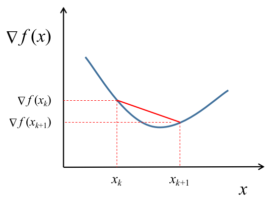
Let $\textbf{B}$ be a matrix estimating the Hessian of our loss function. At iteration $k$, this matrix is deonted by $B_{k}$, when the set of parameters is $x_{k}$ and the gradient of the loss function is $\nabla f(x_{k})$. Then, the following approximation holds true.

For simplicity I will denote $\left(x_{k+1} - x_{k}\right) = s_{k}$ and $\left( \nabla f(x_{k+1}) - \nabla f(x_k) \right) = \textbf{y}_{k}$. This reduces our equation to this form:

For reasons I’m not completely aware of at this point, it is required that $B_{k+1}$ be a symmetric positive definite matrix. There are several ways to represent this condition; one such way of ensuring this is that $s_{k}^{T} B_{k+1} s_{k} > 0$ for all non-zero $s_{k}$. Pre-multiplying the equation above with $s_{k}^{T}$ gives us what is called the curvature condition: $\boxed{s_{k}^{T} y_{k} > 0}$.

Now, we need some way updating this matrix recursively (using past approximations instead of computing it from scratch each time). The method most commonly used is called a Rank 2 update, which uses the following expression for the update.

In this expression, $\textbf{u}$ and $\textbf{v}$ are rank 1 matrices. This means than all rows of $\textbf{u}$ except only one can be expressed as a weighted sum of the other rows (and similarly for $\textbf{v}$). A clever choice of $u=y_{k}$ and $v=B_{k} s_{k}$ is made to preserve the conditions stated earlier. We can derive the expressions for $\alpha$ and $\beta$ as follows. First, we replace $\textbf{u}$ and $\textbf{v}$ in the update equation. Then we pre-multiply by $s_{k}^{T}$ and post-multiply by $\textbf{s}_{k}$ uniformly.

Note that the curvature condition requires the left hand side expression to be positive.

We can choose $\boxed{\alpha=\frac{1}{y_{k}^{T} s_{k}}}$ and $\boxed{\beta = -\frac{1}{s_{k}^{T} B_{k} s_{k}}}$ while preserving the required conditions. Substituting these values along with the others, we get the following update equation for $\textbf{B}$.

But we aren’t satisfied with this. We needed an approximation for the inverse, not the Hessian itself. Fortunately, we have a quick way of getting what we want using the Sherman-Morrison formula. This formula relates the inverse of an updated matrix with the inverse of the matrix itself as follows.

I haven’t been able to perform the complete derivation of the final update expression using this, but the result will be the following.

Example

To illustrate the usage of this solver, I’ll use the minimize function from Python’s open-source scipy.optimize submodule.

import numpy as np
from scipy.optimize import minimize

# Number of examples
N = 100

# Data
x_1 = np.random.normal(5, 1, size=N)
x_2 = np.random.normal(2, 1, size=N)
y = (5*x_1 + 2*x_2 + 5) + np.random.normal(0, 1, size=N)

# Augmented data matrix
Z = np.vstack((np.ones(N), x_1, x_2))

# Loss function to optimize
def mse_loss(params):
    loss = (0.5/N) * (y - params.T.dot(Z)).dot((y - params.T.dot(Z)).T)
    return loss

# Initialize parameters
params_0 = np.zeros((3, 1)) 

# Call the optimizer
res = minimize(mse_loss, params_0, method="BFGS", options={"disp": True})

>>> Optimization terminated successfully.
         Current function value: 0.464744
         Iterations: 8
         Function evaluations: 50
         Gradient evaluations: 10

The optimization completed in 8 iterations and the final loss is about $0.4674$. Users have an option to provide an additional function to compute the derivatives of the loss function, by specifying the jac argument of minimize (jac is shorthand for Jacobian, which is another name for the vector of gradients). Let’s check out the values of estimated parameters. The command below will print the parameters in the format [bias, theta_1, theta_2].

print(res.x)

>>> [4.75559263 5.00640855 1.99609561]

The values estimated by this method are much closer to the real values than those computed by the previous algorithms. Plus, it did so in about half the iterations needed by the previous ones. Several statistical models in Scikit-learn use LBFGS solver by default, which is a limited-memory version of BFGS.

Conclusion

I’m sure I’ve missed out on several details while discussing each of these solvers; the theory behind each of them is very deep and rich, and one could spend several days studying all of it. Even so, I hope this has been a useful headstart for you if you’re delving into the theory of optimization. If any of the facts stated above are inaccurate, please leave a comment below.