Linear Regression from Scratch
Let’s do a silly thought experiment. You’re a student who thinks your scores on a test have some direct relation with the number of hours per week you invest in studying that subject (productive or otherwise). You’ve been making observations for the past 6 tests now, and the data you have looks like this.
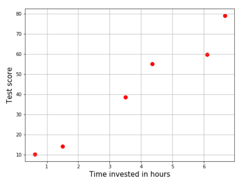
End term exams are closing in and you’ve decided to invest up to 11 hours a week to get your scores up. What maximum score can you expect? If you had a simple equation, say linear, to plug “number of hours” into, you would have an answer. Something like:
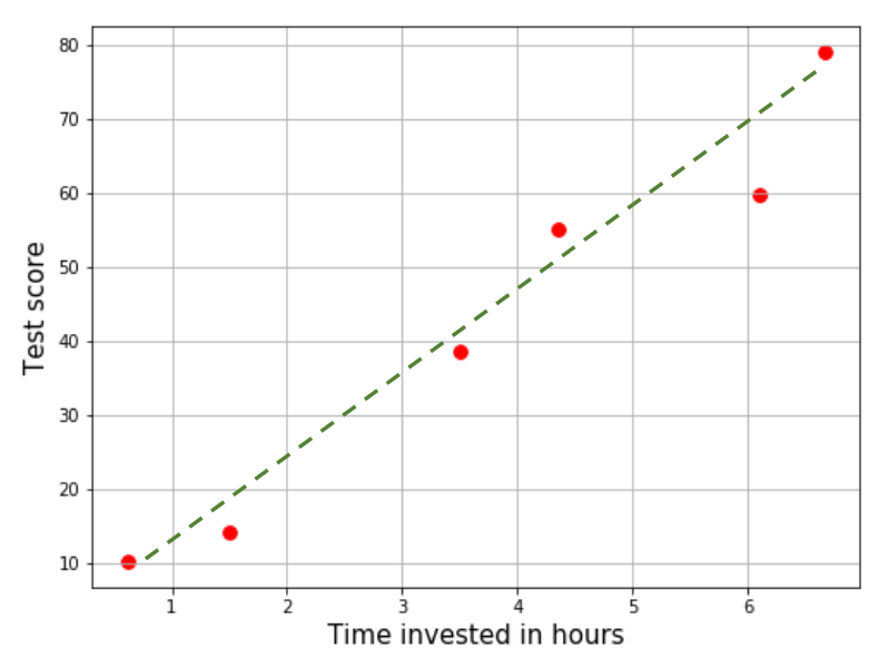
\[\textrm{Expected score} = \left(\textrm{constant 1} \times \textrm{Number of hours}\right) + \textrm{constant 2}\]Sadly, we don’t have such an equation… yet. But by looking at the plot, it does seem like a straight line exists somewhere between those points.
To completely define this line, we must approximate the two constants we saw earlier. The process of estimating such a curve and predicting the values of the dependent variable for unobserved realizations of the independent variable is called regression. If the involved curve has degree 1 (which is entirely our choice), then we can call it linear regression.
The objective
Wait, why are we doing anything else? We do have a line that looks good enough, right? All you would have to do now is extend the line until you can find its projection for 11 hours. And I can go do something else, since we’re done with linear regression.
Not so fast. Try drawing a line for the data below.
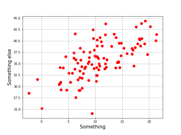
Let me help you out. I’ve drawn three candidate lines. Pick the one that seems best.
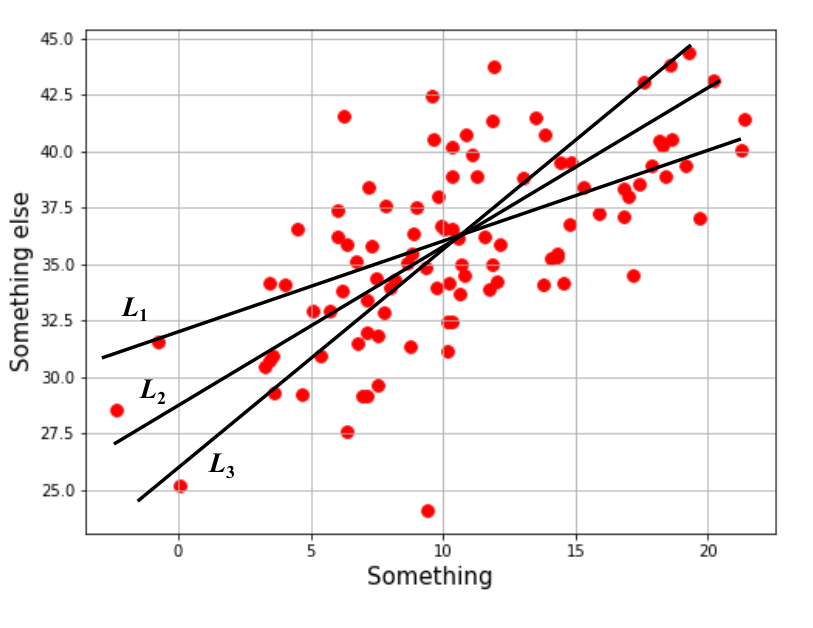
Not so obvious, right? Every person you ask might draw a different line for this data. For an agreeable solution, we must follow a procedure that lands at (roughly) the same solution each time. One way to go about this is to determine how “bad” each solution is and accept the least disappointing one.
Observe that the model’s predictions for known data points differs from the actual output.
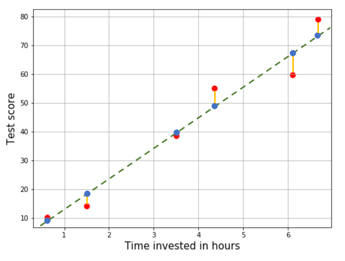
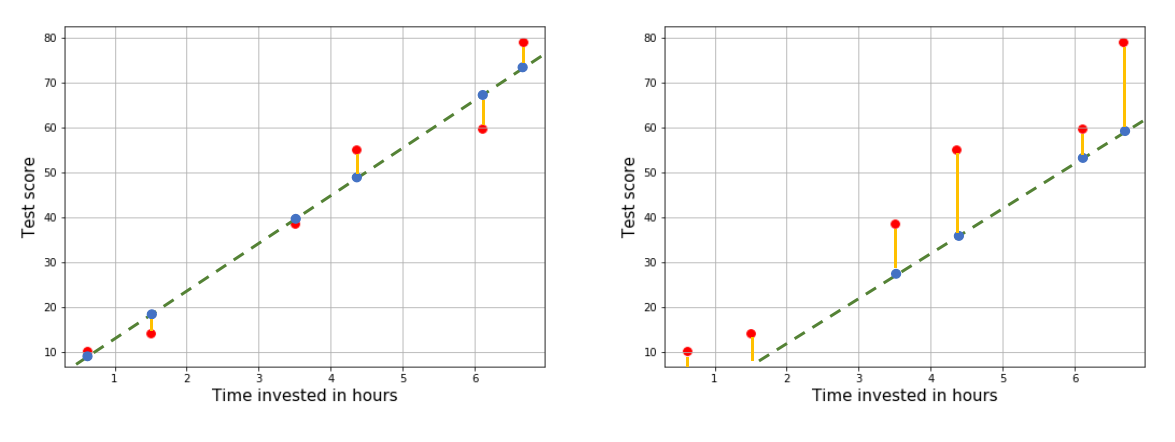
The discrepancy between the actual output (red) and what the line predicts (blue) is the error of prediction. If a model is better than another, it’s “error” should be smaller. In the diagram below, the line on the left is better because it seems to have smaller error than the one on the right.
The next problem we have to deal with is of quantifying this error.
Sum of errors
One naive way of doing this is adding them up. As a convention, let the error be calculated as the actual output (target) minus the prediction. Based on visual estimates, I’ve assigned some error values for our predictions.
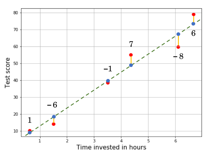
Adding them up, the total error is $-1$. Hmmm… that doesn’t sound right, does it? There’s definitely more error over there than just $-1$, like $+7$ and $-8$. Here’s the problem with this method: if you simply add up all the errors, the positive and negative ones will cancel each other out and the total error will not be representative of all prediction errors.
Sum of absolute errors
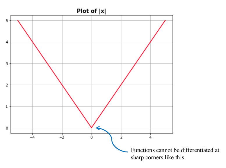
If the sign of the error is our problem, why not disregard it? Either way, positive and negative errors are equally bad for us. If we do that for the above example, the total error is now 29. This method does work, but it doesn’t always converge to the same answer. One of the reasons this happens is because the absolute value function is not differentiable everywhere. Differentiability is a desirable property of error functions.
Sum of squared errors
So we want an error function that disregards the sign of the error, and is differentiable everywhere. Well, squaring a number gets rid of its sign, and the square function is also differentiable everywhere. Seems like we have found what we needed. This function is called the squared error function (duh) and its equation looks like this:
\[\mathcal{L}\left(\hat{y}, y\right)=\frac{1}{2}\sum_{i=1}^{N}\left(y^{(i)}-\hat{y}^{(i)}\right)^{2}\]Here, $y$ represents the model’s target and $\hat{y}$ represents the model’s prediction. The superscript $(i)$ indexes the data points, while $N$ is the total number of data points we have. You might also notice that I represented this function with $\mathcal{L}$. Error functions are often called loss functions, and I’ll be using that name this point forward. Also, I’ve multiplied the sum with $\frac{1}{2}$. You’ll know why soon.
Optimizing the loss function
Let’s come to the main thing. We expect a linear curve to approximate the function generating our data. The linear curve has the following form.
\[\hat{y}(x)=\theta_{0}+\theta_{1}x\]Plugging this into the loss function gives us the equation below.
\[\mathcal{L}=\frac{1}{2}\sum_{i=1}^{N}\left(y^{(i)}-\theta_{0}-\theta_{1}x^{(i)}\right)^{2}\]Note that the only thing we can do to reduce loss (error) is to tune $\theta_{0}$ and $\theta_{1}$ in some way. We do not have any particular idea of what they could actually be, so we initialize them as random numbers. Now if a function depends on a set of variables and we wish to minimze the function by “tuning” those variables, we are performing optimization. What does optimization do?
The plot below shows an example of what a loss function might look like (it’s almost never that smooth in real life).
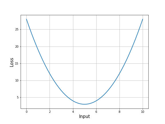
I want you to focus on three points, which I have marked in the next image. Especially, focus on the slope of the loss function curve at those points, which is represented by dotted lines tangent to the curve at those points. The closer the model gets to the right answer, smaller the loss. This tells us that the right answer is likely very close to point $C$.
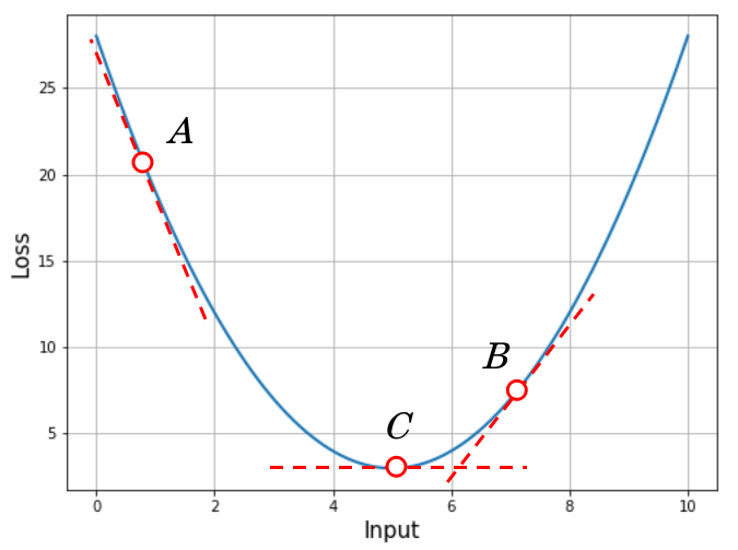
But notice how the slope at point $A$ is very high, that at point $B$ is non-zero but not as high as at $A$, and that at point $C$ is almost zero. This tells us something important: the slope of the loss function at a minimum is close to zero (ideally, exactly zero). The slope of any function at some input is equal to the value of the function’s first derivative at that input. So if we want to find the loss function’s minima, we just have to figure where its first derivative is zero!
We can only tweak $\theta_{0}$ and $\theta_{1}$ in that equation, so the derivative of the loss function will have to be with respect to these two parameters individually. This gives us two equations, shown below.
\[\frac{\partial\mathcal{L}}{\partial\theta_{0}}=\nabla_{\theta_{0}}\left[\frac{1}{2}\sum_{i=1}^{N}\left(y^{(i)}-\theta_{0}-\theta_{1}x^{(i)}\right)^{2}\right]=-\sum_{i=1}^{N}\left(y^{(i)}-\theta_{0}-\theta_{1}x^{(i)}\right)=-\sum_{i}y^{(i)}+\theta_{0}N+\theta_{1}\sum_{i}x^{(i)}\] \[\frac{\partial\mathcal{L}}{\partial\theta_{1}}=\nabla_{\theta_{1}}\left[\frac{1}{2}\sum_{i=1}^{N}\left(y^{(i)}-\theta_{0}-\theta_{1}x^{(i)}\right)^{2}\right]=-\sum_{i=1}^{N}\left(y^{(i)}-\theta_{0}-\theta_{1}x^{(i)}\right)\cdot x^{(i)}=-\sum_{i}x^{(i)}y^{(i)}+\theta_{0}\sum_{i}x^{(i)}+\theta_{1}\sum_{i}\left(x^{(i)}\right)^{2}\]If we hadn’t multiplied by \frac{1}{2} earlier, we would have to carry around the $2$ resulting from the derivative. It doesn’t make a difference if keep it, so it’s up to you. All we have to do now is equate both of them to zero, and solve the equations for $\theta_{0}$ and $\theta_{1}$. How convenient!
\[\theta_{0}N+\theta_{1}\sum_{i}x^{(i)}=\sum_{i}y^{(i)}\] \[\theta_{0}\sum_{i}x^{(i)}+\theta_{1}\sum_{i}\left(x^{(i)}\right)^{2}=\sum_{i}x^{(i)}y^{(i)}\]While there are multiple ways of solving linear equations in two variables, I find it most convenient when the process is vectorized using matrix equations.
\[\left[\begin{array}{cc} N & \sum_{i}x^{(i)}\\ \sum_{i}x^{(i)} & \sum_{i}\left(x^{(i)}\right)^{2} \end{array}\right]\left[\begin{array}{c} \theta_{0}\\ \theta_{1} \end{array}\right]=\left[\begin{array}{c} \sum_{i}y^{(i)}\\ \sum_{i}x^{(i)}y^{(i)} \end{array}\right]\]So our solution is simply …
\[\left[\begin{array}{c} \theta_{0}\\ \theta_{1} \end{array}\right]=\left[\begin{array}{cc} N & \sum_{i}x^{(i)}\\ \sum_{i}x^{(i)} & \sum_{i}\left(x^{(i)}\right)^{2} \end{array}\right]^{-1}\left[\begin{array}{c} \sum_{i}y^{(i)}\\ \sum_{i}x^{(i)}y^{(i)} \end{array}\right]\]Let’s generate some dummy data for regression and see what kind of result this method gives us.
import numpy as np
import matplotlib.pyplot as plt

x = np.random.normal(5, 10, size=50)
y = (0.5 * x + 8) + np.random.normal(0, 2, size=50)
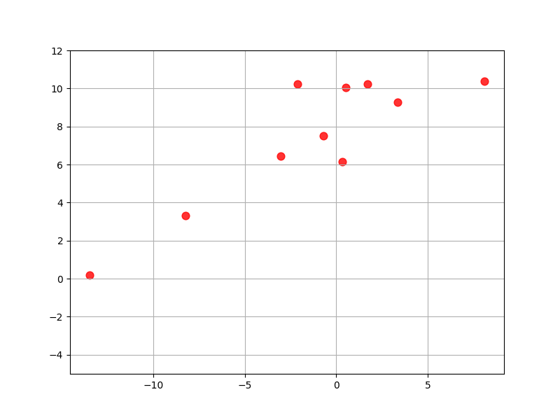
Note that the line we have generated is $y=0.5x + 8$. I’ve added some Gaussian noise to make it slightly more realistic. When rendered on a scatter plot, the data looks like the plot shown below. What you get might differ from mine, since I am generating random numbers.
Next, let’s define the two matrices we need for computing the values of our parameters.
# Coefficients matrix
A = np.array([[50, np.sum(x)],
              [np.sum(x), np.sum(x**2)]])

# Constants matrix
b = np.array([[np.sum(y)],
              [np.sum(x*y)]])
Ensure that the matrices have the right dimensions. $A$ should be $(2 \times 2)$ and $b$ should be $(2 \times 1)$. You can check this using the shape attribute of NumPy arrays. All that’s left is to solve the equation!
# Solve the matrix equation
thetas = np.linalg.inv(A).dot(b)

# Check the answer
print(thetas)
>>> [[7.95271631]
     [0.4786904 ]]
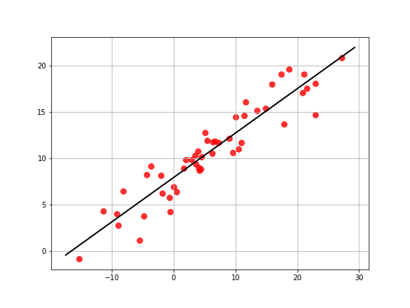
The algorithm has evaluated $\theta_{0}=7.95$ and $\theta_{1}=0.48$. That’s really close to the true values. Looks like it worked! Let’s plot the line on the data to see what it looks like.
plt.figure(figsize=(8, 6))

# Plot the points
plt.scatter(x, y, color='red', s=60, marker='o', alpha=0.8)

# Get coordinates of the line's ends
x1, x2 = plt.xlim()
y1, y2 = thetas[0] + thetas[1] * x1, thetas[0] + thetas[1] * x2

# Plot the line
plt.plot([x1, x2], [y1, y2], color='black', linewidth=2)

# Other layout options
plt.grid()
plt.show()
Multivariate linear regression
What if your output variable depends on more than one independent variable? Let’s say our experiment from earlier now depends not only on the number of hours invested but also on the quantity of food you consume during that period (I’ve generated random numbers for demo purposes). The points now lie on a surface, as shown below.
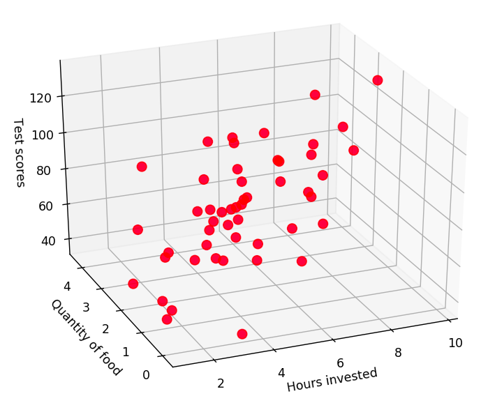
The equation now governing our output might be something like this.
\[\hat{y}^{(i)}=\theta_{0}+\theta_{1}x_{1}^{(i)}+\theta_{2}x_{2}^{(i)}\]We could go through the entire procedure again and get another matrix equation to solve, which will work. Instead, let’s generalize this process to any number of variables. That is, let’s say our inputs are now $n$ dimensional vectors, where each element is a feature of the input (like hours invested and quantity of food).
\[\textbf{x}^{(i)}=\left[\begin{array}{c} x_{1}^{(i)}\\ x_{2}^{(i)}\\ \vdots\\ x_{n}^{(i)} \end{array}\right]\]The equation governing the output would look like the one shown below, which can be arranged into a vectorized expression easily.
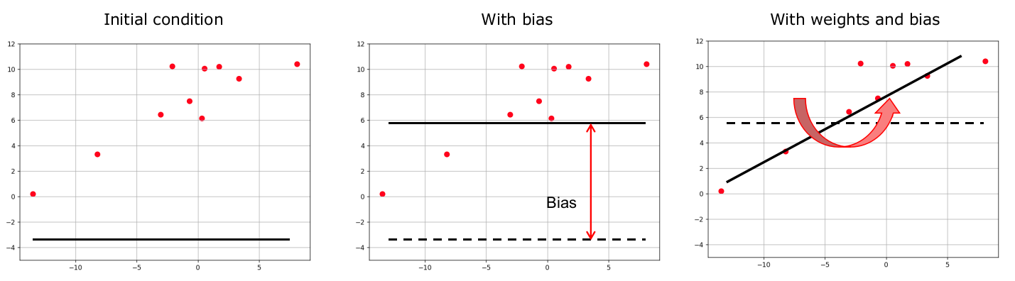
\[\hat{\textbf{y}}^{(i)}=\theta_{0}+\theta_{1}x_{1}^{(i)}+\theta_{2}x_{2}^{(i)}+...+\theta_{n}x_{n}^{(i)}=\theta_{0}+\left[\begin{array}{cccc} \theta_{1} & \theta_{2} & ... & \theta_{n}\end{array}\right]\left[\begin{array}{c} x_{1}^{(i)}\\ x_{2}^{(i)}\\ \vdots\\ x_{n}^{(i)} \end{array}\right]=\textbf{w}^{T}\textbf{x}^{(i)}+b\] \[\textrm{where}\quad\textbf{w}=\left[\begin{array}{c} \theta_{1}\\ \theta_{2}\\ \vdots\\ \theta_{n} \end{array}\right]\quad\textrm{and}\quad\theta_{0}=b\]I’ve renamed some variables here. First, the vector of coefficients is now $\textbf{w}$ and is called the vector of weights. $\theta_{0}$ is now $b$ and is called the bias. They are named so because the weights (loosely) determine the importance of each variable in the prediction and the bias offsets the predicted surface by some distance. In a way, the bias helps position the surface in the correct location and the weights help tilt the surface to the right orientation.
Let’s compute the gradients of the prediction function before hand. The parameters we can change are all the elemnts of $\textbf{w}$ and $b$. Given that $\hat{\textbf{y}}=b+\theta_{1}x_{1} + \theta_{2}x_{2} + … + \theta_{n}x_{n}$, we have:
\[\frac{\partial\hat{y}}{\partial\theta_{1}}=\nabla_{\theta_{1}}\left(\theta_{0}+\theta_{1}x_{1}+...+\theta_{n}x_{n}\right)=x_{1}\] \[\frac{\partial\hat{y}}{\partial\theta_{2}}=\nabla_{\theta_{2}}\left(\theta_{0}+\theta_{1}x_{1}+...+\theta_{n}x_{n}\right)=x_{2}\] \[\frac{\partial\hat{y}}{\partial\theta_{n}}=\nabla_{\theta_{n}}\left(\theta_{0}+\theta_{1}x_{1}+...+\theta_{n}x_{n}\right)=x_{n}\]We can vectorize this as follows.
\[\nabla_{\textbf{w}}\hat{\textbf{y}}=\left[\begin{array}{c} \frac{\partial\hat{y}}{\partial\theta_{1}}\\ \frac{\partial\hat{y}}{\partial\theta_{2}}\\ \vdots\\ \frac{\partial\hat{y}}{\partial\theta_{n}} \end{array}\right]=\left[\begin{array}{c} x_{1}\\ x_{2}\\ \vdots\\ x_{n} \end{array}\right]=\textbf{x}\quad\textrm{and}\quad\nabla_{b}\hat{\textbf{y}}=\frac{\partial\hat{\textbf{y}}}{\partial\theta_{0}}=1\]Now, we can differentiate our loss function with respect to the weights and bias which will give us the required equation to solve for the minimum.
\[\nabla_{\textbf{w}}\mathcal{L}=\nabla_{\textbf{w}}\left[\frac{1}{2}\sum_{i=1}^{n}\left(y^{(i)}-\textbf{w}^{T}\textbf{x}^{(i)}-b\right)^{2}\right]=-\sum_{i=1}^{N}\left(y^{(i)}-\textbf{w}^{T}\textbf{x}^{(i)}-b\right)\cdot\nabla_{\textbf{w}}\left[\textbf{w}^{T}\textbf{x}^{(i)}+b\right]=-\sum_{i=1}^{N}\left(y^{(i)}-\textbf{w}^{T}\textbf{x}^{(i)}-b\right)\cdot\textbf{x}^{(i)}\] \[\nabla_{b}\mathcal{L}=\nabla_{b}\left[\frac{1}{2}\sum_{i=1}^{n}\left(y^{(i)}-\textbf{w}^{T}\textbf{x}^{(i)}-b\right)^{2}\right]=-\sum_{i=1}^{N}\left(y^{(i)}-\textbf{w}^{T}\textbf{x}^{(i)}-b\right)\cdot\nabla_{b}\left[\textbf{w}^{T}\textbf{x}^{(i)}+b\right]=-\sum_{i=1}^{N}\left(y^{(i)}-\textbf{w}^{T}\textbf{x}^{(i)}-b\right)\]The first equation gives a vector with the same dimensions as the weights. The second equation gives a scalar value. What we now have to solve is this.
\[\sum_{i=1}^{N}\left(y^{(i)}-\textbf{w}^{T}\textbf{x}^{(i)}-b\right)\cdot\textbf{x}^{(i)}=0\quad\textrm{and}\quad\sum_{i=1}^{N}\left(y^{(i)}-\textbf{w}^{T}\textbf{x}^{(i)}-b\right)=0\]Solving this pair of equations is not straightforward (for me), so let’s make some simplifications. First, let’s assume that there’s only one data point. Second, let’s assume that every input vector has only 2 features. These modifications help us simplify those two equations as follows.
\[\left(y-\theta_{1}x_{1}-\theta_{2}x_{2}-b\right)\left[\begin{array}{c} x_{1}\\ x_{2} \end{array}\right]=0\quad\Rightarrow\quad\begin{cases} yx_{1}-\theta_{1}x_{1}^{2}-\theta_{2}x_{1}x_{2}-bx_{1}=0\\ yx_{2}-\theta_{1}x_{1}x_{2}-\theta_{2}x_{2}^{2}-bx_{2}=0 \end{cases}\] \[y-\theta_{1}x_{1}-\theta_{2}x_{2}-b=0\]Like before, we can combine all three into a matrix equation like so:
\[\left[\begin{array}{ccc} 1 & x_{1} & x_{2}\\ x_{1} & x_{1}^{2} & x_{1}x_{2}\\ x_{2} & x_{1}x_{2} & x_{2}^{2} \end{array}\right]\left[\begin{array}{c} b\\ \theta_{1}\\ \theta_{2} \end{array}\right]=\left[\begin{array}{c} y\\ yx_{1}\\ yx_{2} \end{array}\right]\]… which can be vectorized as follows.
\[\left[\begin{array}{c} 1\\ x_{1}\\ x_{2} \end{array}\right]\left[\begin{array}{ccc} 1 & x_{1} & x_{2}\end{array}\right]\cdot\left[\begin{array}{c} b\\ \theta_{1}\\ \theta_{2} \end{array}\right]=\left[\begin{array}{c} 1\\ x_{1}\\ x_{2} \end{array}\right]\cdot\left[y\right]\] \[\left(\textbf{z}\cdot\textbf{z}^{T}\right)\cdot\Theta=\textbf{z}\cdot y\quad\textrm{where}\quad\textbf{z}=\left[\begin{array}{c} 1\\ x_{1}\\ \vdots\\ x_{n} \end{array}\right]\;;\;\Theta=\left[\begin{array}{c} b\\ \theta_{1}\\ \vdots\\ \theta_{n} \end{array}\right]\]This very same expression works for data with more than one data points as well. The nature of matrix multiplication makes everything fall right in place. The expression for computing our parameters is summarized below.
\[\left(\textbf{Z}\cdot\textbf{Z}^{T}\right)\cdot\Theta=\textbf{Z}\cdot\textbf{y}\quad\textrm{where}\quad\textbf{Z}=\left[\begin{array}{ccc} 1 & ... & 1\\ x_{1}^{(1)} & & x_{1}^{(N)}\\ x_{2}^{(1)} & \ddots & x_{2}^{(N)}\\ \vdots & & \vdots\\ x_{n}^{(1)} & \dots & x_{n}^{(N)} \end{array}\right]\;;\;\textbf{y}=\left[\begin{array}{ccc} y^{(1)} & ... & y^{(N)}\end{array}\right]\;;\;\Theta=\left[\begin{array}{c} b\\ \theta_{1}\\ \vdots\\ \theta_{n} \end{array}\right]\]Let’s get that to work on some data. The data on the plot at the beginning of this section was generated using the code below.
import numpy as np

x_1 = np.random.normal(5, 1, size=50)
x_2 = np.random.normal(2, 1, size=50)
y = 5*x_1 + 2*x_2 + 10 + np.random.normal(0, 1, size=50)
Next, we can compute each matrix separately and combine them to solve the equation.
# Create z by padding [x_1, x_2] with ones
z = np.vstack((np.ones(50), x_1, x_2))

# Coefficient matrix
A = z.dot(z.T)

# Constant matrix
b = z.dot(y.reshape(-1, 1))

# Get parameter values
param_vector = np.linalg.inv(A).dot(b)

print(param_vector)
>>> [[10.08439479]
     [ 5.00964836]
     [ 1.94088811]]
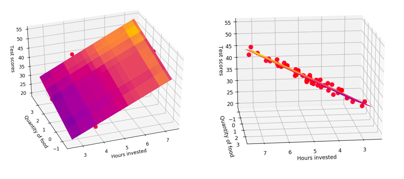
As expected, the estimates $b=10.08$, $\theta_{1}=5.01$ and $\theta_{2}=1.94$ are really close to the true values. Why are they not exactly equal? That happens due to the noise in the system. If we increase the magnitudes of noise, the values will stray further away from the truth. Before moving on, let’s see what our prediction surface looks like.
# Intialize figure and plot the data points
fig = plt.figure(figsize=(8, 6))
ax = fig.add_subplot(projection='3d')
ax.scatter(x_1, x_2, y, s=60, color='red', alpha=0.7, marker='o')

# Create meshgrids for features and output ...
# ... and render them using plot_surface
xx_1, xx_2 = np.meshgrid(x_1, x_2)
yy = param_vector[0] + param_vector[1]*xx_1 + param_vector[2]*xx_2
ax.plot_surface(xx_1, xx_2, yy, cmap='plasma', alpha=0.5)

# Layout options
ax.set_xlabel("Hours invested")
ax.set_ylabel("Quantity of food")
ax.set_zlabel("Test scores")
plt.show()
Iterative methods for regression
Didn’t I say earlier that we’re generalizing our equations? Why another method now? In all the computations we performed above, I quietly swept something under the carpet: the small size of our data. While this method gives us answers in one shot and is pretty accurate, it has a major drawback. The computations of the parameter vector involves computing the inverse of a matrix, which (effort wise) isn’t easy for your computer. That is because this operation evolves with $\mathcal{O}(n^{3})$ in time. This means, if you double the size of your data, it’ll take $2^{3}=8$ times longer to finish the computation of the matrix inverse. Typically, your data will contain thousands of records each with hundreds of features. And that’ll be way too much time for such a simple algorithm.
When we cannot land at an exact solution, we resort to approximation. These approximations are done iteratively, by evaluation at each stage how good the model is doing and what changes must be made next to make it perform even better.
Here’s some visual intuition of what we are going to do. Remember the overly simplified loss surface from earlier? All this time, we were using the fact that the slope of this function at the minimum is zero, and we would find the set of parameters that would satisfy this condition. This time, our startegy is different.
- Start at some random location on the loss surface. This is simply done by randomly initializing the paramter vector
- Compute the slope (gradient) of the loss function at this point.
- If the curve is locally going upwards (left to right), then the minimum is likely somewhere on your left. Take a small step to your left, commensurate with the magnitude of slope. Instead, of the curve is locally moving downwards (left to right), then the minimum could be somewhere ahead of you. Take a small step to your right in a similar way.
- In the new position, compute the slope again and repeat the process until the slope becomes small enough or you reach the iteration limit.
Here’s what happens on the curve when we perform this process.
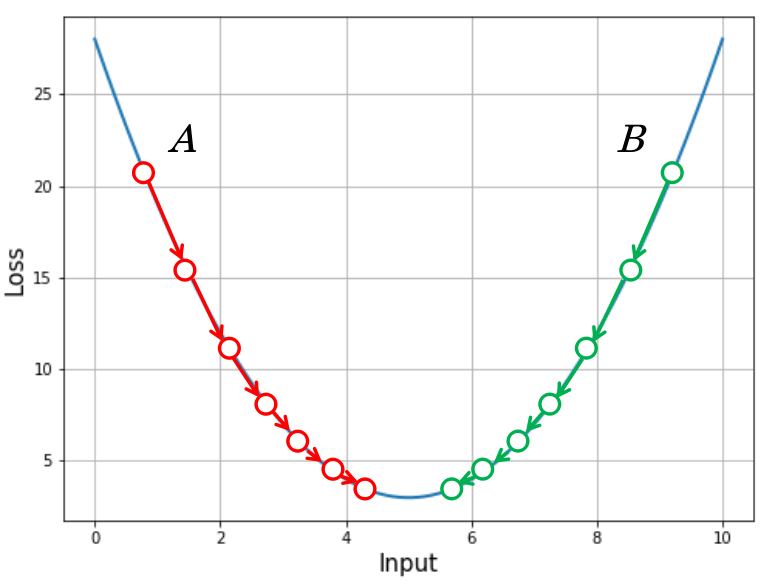
If you start at point A, the slope is high and negative. You take a good step in the positive direction, which reduces the loss and the slope at the new point. From here you take a step that’s a little smaller, since the slope here is not as high. Going on like this, you come very close to the minimum where the slopes are really small and your steps aren’t large enough to make any significant progress. That’s where the model has converged.
The updates to the parameters for generating this behavior is handled through the following equation.
\[\Delta\Theta=-\eta\frac{\partial\mathcal{L}}{\partial\Theta}\quad\Rightarrow\quad\Theta:=\Theta-\eta\frac{\partial\mathcal{L}}{\partial\Theta}\]In that, $\eta$ is called the learning rate, which is usually a small value like $0.01$. This hyperparameter directly affects the size of the step taken at each iteration. This equation does exactly what we saw before. When the slope of the loss function at a point is positive (like point $B$), $\Delta \Theta$ becomes negative and the parameter value reduces. When at a location like point $A$, the slope is negative, $\Delta \Theta$ becomes positive and the parameter value increases. It is easy to determine the expression for $\frac{\partial \mathcal{L}}{\partial \Theta}$.
\[\frac{\partial\mathcal{L}}{\partial\Theta}=\nabla_{\Theta}\left[\frac{1}{2N}\sum_{i=1}^{N}\left(\textbf{y}^{(i)}-\Theta^{T}\textbf{z}^{(i)}\right)^{2}\right]=-\frac{1}{N}\sum_{i=1}^{N}\left(\textbf{y}^{(i)}-\Theta^{T}\textbf{z}^{(i)}\right)\cdot\textbf{z}^{(i)}\]Notice that I’ve also divided by $N$, i.e. I’ve averaged the loss instead of just summing it up. This is done to reduce the magnitude of the gradient, which helps in stable movement along the loss curve. Therefore, the update equation becomes:
\[\Theta:=\Theta+\frac{\eta}{N}\sum_{i=1}^{N}\left(\textbf{y}^{(i)}-\Theta^{T}\textbf{z}^{(i)}\right)\cdot\textbf{z}^{(i)}\]Here’s some code to get this to work.
import numpy as np

# Number of samples
N = 100

x_1 = np.random.normal(5, 1, size=N)
x_2 = np.random.normal(2, 1, size=N)
y = 5*x_1 + 2*x_2 + 5 + np.random.normal(0, 1, size=N)

# Create z matrix
z = np.vstack((np.ones(N), x_1, x_2))

# Randomly initialize the parameter vector
# It will be a vector of size (3, 1)
params = np.random.uniform(0, 5, size=(3, 1))

# Learning is a parameter we can control
# I'm setting it to 0.05
eta = 0.05

# We'll perform 20 updates in a loop
iters = 20

for i in range(iters):

    # Update equation
    params += (eta/N)*((y - params.T.dot(z)) * z).sum(axis=1).reshape(-1, 1)

    # Let's also compute the loss at each stage
    # I'll print it every 10 iterations
    loss = (1/(2*N))*((y - params.T.dot(z))**2).sum(axis=1)[0]
    print("Iteration {:2d} - MSE Loss {:.4f}".format(i, loss))

# Print final parameter values
print("\nFinal parameter values:")
print("----------------------------------------")
print("theta_1: {:.2f}".format(params[1][0]))
print("theta_2: {:.2f}".format(params[2][0]))
print("bias: {:.2f}".format(params[0][0]))
>>> Iteration  0 - MSE Loss 4.7369
    Iteration  1 - MSE Loss 3.9087
    Iteration  2 - MSE Loss 3.2518
    Iteration  3 - MSE Loss 2.7297
    Iteration  4 - MSE Loss 2.3138
    Iteration  5 - MSE Loss 1.9817
    Iteration  6 - MSE Loss 1.7159
    Iteration  7 - MSE Loss 1.5026
    Iteration  8 - MSE Loss 1.3308
    Iteration  9 - MSE Loss 1.1920
    Iteration 10 - MSE Loss 1.0796
    Iteration 11 - MSE Loss 0.9882
    Iteration 12 - MSE Loss 0.9136
    Iteration 13 - MSE Loss 0.8524
    Iteration 14 - MSE Loss 0.8022
    Iteration 15 - MSE Loss 0.7606
    Iteration 16 - MSE Loss 0.7262
    Iteration 17 - MSE Loss 0.6976
    Iteration 18 - MSE Loss 0.6736
    Iteration 19 - MSE Loss 0.6536

    Final parameter values:
    ----------------------------------------
    theta_1: 4.98
    theta_2: 2.44
    bias: 4.05
Although the estimates aren’t as good as our previous methods, they’re close enough. If you run this several times, you’ll notice that this method doesn’t provide very stable training (diregarding the fact that different set of data points are generated each time). Several improvements to this model have been made over time. One such improvement is the use of second order derivative information, which I will discuss in an upcoming post. Meanwhile, I hope this post has been a good resource for you to understand linear regression.