Model Complexity and Regularization

06 September 2020 - 35 mins read time
Tags: Calculus Linear Algebra Python

So far we’ve looked at data where the features were linearly related to the target, such that the approximated function could be represented as follows.

However, that won’t happen all the time. Consider the univariate data shown below.

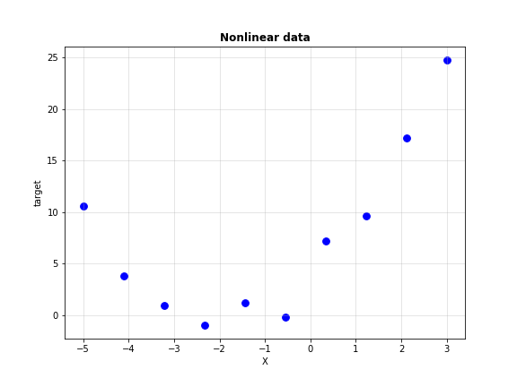
Not very linear now, is it? Clearly, we need higher order features to model this regression task. This form of regression is called Polynomial Regression. Linear regression is a special case of polynomial regression where our features have degree 1.

Polynomial Regression

Say you suspect that the target has quadratic (degree 2) dependence on the features. Now if your data had two features, $x_{1}$ and $x_{2}$, you don’t know which feature exactly it depends quadratically on. What we do is generate higher degree features right from degree 0 (constant) to degree 2. That is, for the following features will be generated.

With the six features we generated, our approximated function now looks like this.

Notice that the weight associated with constant feature $1$ is the bias term $\theta_{0}$. After regression is performed using this function, the magnitudes of the coefficients will tell us which polynomial term affects the target most. Let’s write some code to get this working.

Before we proceed from here, I need to tell you that I’m changing my notation a little bit. Earlier, we would treat our features as a matrix with $n$ rows and $m$ columns, where $m$ was the number of data points and $n$ was the number of features. Henceforth, I’ll represent this as a matrix of size $m \times n$ instead, with $m$ rows and $n$ columns. This brings to the form data will usually be available in the real world: data points as rows and columns as features. Accordingly, the prediction function changes to the following, given a data matrix $X$ and weight vector $\Theta$.

To generate the polynomial features, I’m going to use PolynomialFeatures class from sklearn.preprocessing submodule. Here’s some code to give you an example of how it works.

import numpy as np
from sklearn.preprocessing import PolynomialFeatures

poly = PolynomialFeatures(degree=2)

# Create an array with 4 rows and 2 columns
x = np.array([[1, 2], 
              [3, 4],
              [0, 1],
              [2, 3]])

# Fit and transform x using poly to get the features
x_poly = poly.fit_transform(x)

# Print both
print("Original data")
print(x)

print("\nData with polynomial features added")
print(x_poly)

>>> Original data
    [[1 2]
     [3 4]
     [0 1]
     [2 3]]

    Data with polynomial features added
    [[ 1.  1.  2.  1.  2.  4.]
     [ 1.  3.  4.  9. 12. 16.]
     [ 1.  0.  1.  0.  0.  1.]
     [ 1.  2.  3.  4.  6.  9.]]

We’ll first perform linear regression on the data without polynomial features, and then again after generating polynomial features of degree 2 (since we suspect quadratic independence). To perform linear regression, we will now use the LinearRegression class from sklearn.linear_model submodule. Here’s the regression model without polynomial features.

import numpy as np
import matplotlib.pyplot as plt
from sklearn.linear_model import LinearRegression

np.random.seed(1)

# The data 
# Sklearn requires the data to be of shape (m, n)
x = np.linspace(-5, 3, 10).reshape(-1, 1)
y = (x+2)**2 + np.random.normal(0, 1, 10)

# Initialize a linear regression object
linreg = LinearRegression()

# Fit the model on the data
# This makes it learn the coefficients
linreg.fit(x, y)

# Predict on x to get the predicted values of x
y_pred = linreg.predict(x)

Here’s the code with polynomial features added.

import numpy as np
import matplotlib.pyplot as plt
from sklearn.linear_model import LinearRegression
from sklearn.preprocessing import PolynomialFeatures

np.random.seed(1)

# Polynomial features object
poly = PolynomialFeatures(degree=2)

# The data 
# Sklearn requires the data to be of shape (m, n)
x = np.linspace(-5, 3, 10).reshape(-1, 1)
y = (x+2)**2 + np.random.normal(0, 1, 10).reshape(-1, 1)
x_poly = poly.fit_transform(x)

# Initialize a linear regression object
linreg_poly = LinearRegression()

# Fit the model on the data
# This makes it learn the coefficients
linreg_poly.fit(x_poly, y)

# Predict on x to get the predicted values of x
y_pred_poly = linreg_poly.predict(x_poly)

Let’s plot the predictions with the data to see which one’s done better.

def plot_regression(X, y_true, y_pred, y_pred_poly):
    
    # We have to sort the predictions by X
    # To make the plot look right
    X = X.reshape(len(X),)
    y_true = y_true.reshape(len(y_true),)
    y_pred = y_pred.reshape(len(y_pred),)
    y_pred_poly = y_pred_poly.reshape(len(y_pred_poly),)
    
    # Sort 
    ranks = np.argsort(X)
    X = X[ranks]
    y_true = y_true[ranks]
    y_pred = y_pred[ranks]
    y_pred_poly = y_pred_poly[ranks]
    
    # Plot the predictions
    fig = plt.figure(figsize=(16, 6))
    ax1 = fig.add_subplot(121)
    ax1.scatter(X, y_true, s=60, color='b', label='Data')
    ax1.plot(X, y_pred, color='k', linewidth=2, label='Prediction')
    ax1.grid(alpha=0.3)
    ax1.legend()
    ax1.set_title("Without polynomial features", fontweight='bold')
    
    ax2 = fig.add_subplot(122)
    ax2.scatter(X, y_true, s=60, color='b', label='Data')
    ax2.plot(X, y_pred_poly, color='k', linewidth=2, label='Prediction')
    ax2.grid(alpha=0.3)
    ax2.legend()
    ax2.set_title("With polynomial features", fontweight='bold')
    
    plt.tight_layout(pad=3)
    plt.savefig("poly_regression.png")
    plt.show()

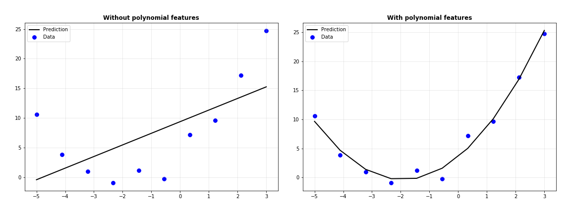
Clearly, the polynomial features have helped fit the data better. Let’s analyze the coefficients of the regressor where polynomial features were used.

print(linreg_poly.coef_)

>>> [[0.         4.07914898 1.06080172]]

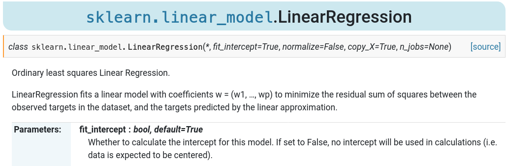
The features in our data were in the order $1$, $x$, $x^{2}$, which means the approximated function must look like $1.06x^{2} + 4.07x$. Note that the original function we used is $(x+2)^{2}=x^{2} + 4x + 4$. Why is the bias zero? A quick look at LinearRegression documentation reveals that the class has a parameters fit_intercept set to True by default. The model will compute the bias on its own, which is why it ignores the bias feature we gave it (the column doesn’t provide any information anyway since it’s only full of 1’s).

You can check the bias estimated by the model by using the intercept_ attribute of the regressor.

print(linreg_poly.intercept_)

>>> [3.52486922]

It’s close to 4 as expected, deviating away only due to the noise we added to the system.

What happens at higher degrees?

We used second degree features because the curve looked quadratic. What if we cannot estimate the degree of the polynomial by just looking at the data? One way out of this is a bruteforce solution: we try different degrees of polynomials until the fit looks good enough. The fit will be good enough when the squared error loss is sufficiently small. Let’s implement this idea and see what happens. Specifically, I’m going to reuse the data from above and fit 9 polynomials to it, starting from degree 1 to degree 9. I’ll compute the squared error loss (using mean_squared_error from sklearn.metrics) for each model by predicting on the data we have and finally, plot the losses for each degree.

import numpy as np
import matplotlib.pyplot as plt
from sklearn.linear_model import LinearRegression
from sklearn.preprocessing import PolynomialFeatures
from sklearn.metrics import mean_squared_error 

np.random.seed(1)

# The data
x = np.linspace(-5, 3, 10).reshape(-1, 1)
y = (x+2)**2 + np.random.normal(0, 1, 10).reshape(-1, 1)

# List to store losses
losses = []

# Loop over degree 1 to 9
for deg in range(1, 10):
    
    # Polynomial features object
    poly = PolynomialFeatures(degree=deg)

    # Generate polynomial features
    x_poly = poly.fit_transform(x)

    # Initialize a linear regression object
    linreg_poly = LinearRegression()

    # Fit the model on the data
    # This makes it learn the coefficients
    linreg_poly.fit(x_poly, y)

    # Predict on x to get the predicted values of x
    y_pred_poly = linreg_poly.predict(x_poly)
    
    # Compute mean squared error and append to losses
    loss = mean_squared_error(y, y_pred_poly)
    losses.append(loss)
    
    
# Plot the losses
plt.figure(figsize=(8, 6))
plt.plot([i for i in range(1, 10)], losses, color='b', marker='o')
plt.xlabel("Degree")
plt.ylabel("MSE Loss")
plt.title("MSE loss vs. degree of polynomial", fontweight='bold')
plt.grid(alpha=0.3)
plt.savefig("loss_vs_degree.png")
plt.show()

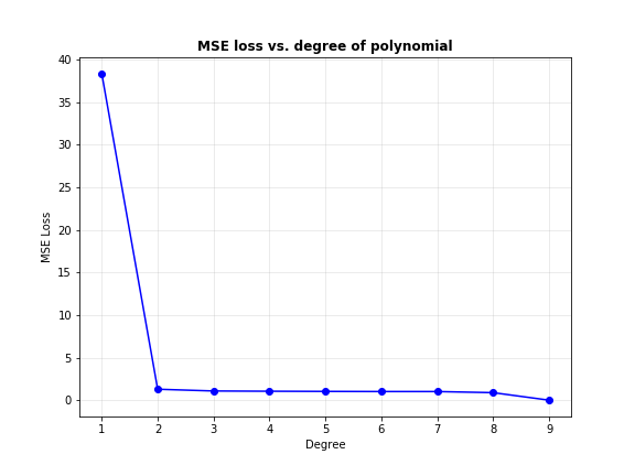
Interesting. As the degree of the polynomial increases, the loss seems to keep going down: quickly from degree 1 to 2, and gradually thereafter. Below, I’ve plot the predicted curves for degree 2, 3, 6 and 9.

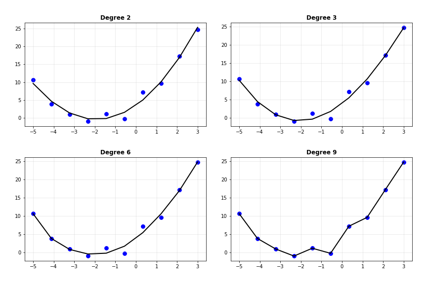
Notice how the curve slowly begins passing through every single data point as the degree increases, such that it passes through every single point when the degree is 9. Does that mean we can use even more complex models to get better predictions?

Let’s perform a sanity check. This time, I’ll train on the data that we already have but predict on a new set of data points, which the model has never seen. Traditionally, the data used to learn the model parameters is called the training dataset and the new one we’re generating is called the validation, development or evaluation dataset. You might see the term test dataset being used in many places, but the purpose of test data is wholly different.

Let’s generate some new data and retrain all the models. This time, I’ll plot the predictions on the training data and on the validation data for degrees 2, 6 and 9 side by side.

import numpy as np
import matplotlib.pyplot as plt
from sklearn.linear_model import LinearRegression
from sklearn.preprocessing import PolynomialFeatures
from sklearn.metrics import mean_squared_error 

np.random.seed(1)

# Training data
X_train = np.linspace(-5, 3, 10).reshape(-1, 1)
y_train = (X_train + 2)**2 + np.random.normal(0, 1, 10).reshape(-1, 1)

# Validation data
# Sorting it so that plotting is easier
X_val = np.sort(np.random.uniform(-5, 3, size=5)).reshape(-1, 1)
y_val = (X_val + 2)**2 + np.random.normal(0, 1.2, 5).reshape(-1, 1)

# List to store losses
train_losses = []
val_losses = []

# List to store predictions
train_predictions = []
val_predictions = []

# Loop over degree 1 to 9
for deg in range(1, 10):
    
    # Polynomial features object
    poly = PolynomialFeatures(degree=deg)

    # Generate polynomial features
    X_poly_train = poly.fit_transform(X_train)
    X_poly_val = poly.fit_transform(X_val)

    # Initialize a linear regression object
    linreg_poly = LinearRegression()

    # Fit the model on the data
    # This makes it learn the coefficients
    linreg_poly.fit(X_poly_train, y_train)

    # Predict on training and validation data
    train_preds = linreg_poly.predict(X_poly_train)
    val_preds = linreg_poly.predict(X_poly_val)
    
    train_predictions.append(train_preds)
    val_predictions.append(val_preds)
    
    # Compute mean squared error and append to losses
    train_loss = mean_squared_error(y_train, train_preds)
    train_losses.append(train_loss)
    val_loss = mean_squared_error(y_val, val_preds)
    val_losses.append(val_loss)

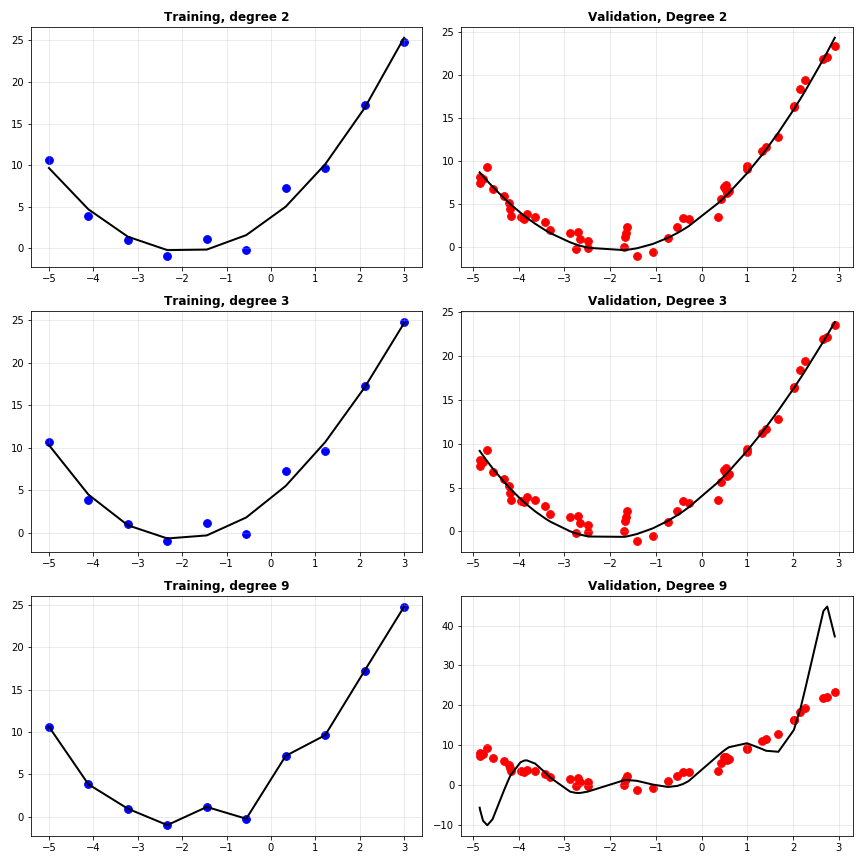
Interesting again. Note how the second degree polynomial fits the validation data just fine, the degree 6 polynomial is okay but slightly off compared to degree 2, and degree 9 is total chaos. Let’s have a look at the training and validation MSE losses of the models.

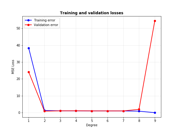
A good model is one that performs equally well on training and validation data. From the plot above, we can conclude that neither very low degrees (like 1) or very high degrees (like 9) make good models for this data, since the gap between their train and validation errors are high. The sweet spot lies somewhere between 2 to 8, which the reader may choose as the one with minimum gap between the two errors. However, it is clear that goodness of fit cannot be determined by monitoring training loss alone: validation loss is equally important.

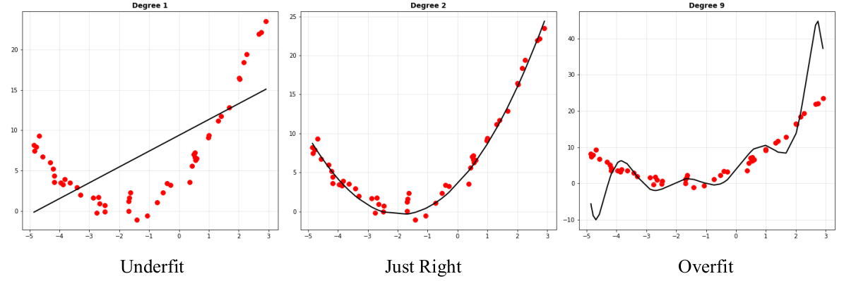
Either way, why were very complex models unable to fit the data well? Every feature added to the data provides the model a deeper understanding of the underlying patterns in the data. However, if there are too many features, the model learns more patterns than it should: it learns to model the noise in the data as well. This is not good, since noise is random and distracting for the model. Noise learnt on the training data could be different from that in the validation data, which will make model predictions really bad.

Aptly, this phenomenon is known as overfitting: the model fits the data unnecessarily well. A contrasting phenomenon was seen on the linear model (degree 1): the model fails to capture the required pattern and underfits the data. Increasing complexity takes the model from the underfitting zone, to a sweet spot, then to the overfitting zone. Our job is to find the sweet spot (or get as close to it as possible).

Bias and Variance: model consistency

Suppose you have a large dataset with several thousand data points, generated by the same distribution. You randomly sample 100 points from this set and fit a model to it. Then you predict on the validation set. You perform this several times and plot all of the predicted curves together. Will you get the exact same curve each time? You might have guessed that we won’t, and you’re right. The approximated function is dependent on the data you have, and it will change to some degree when the data changes. The next obvious question is whether we know to what extent the model will change when the data changes. Let’s perform the experiment stated above to find out.

import numpy as np
from sklearn.linear_model import LinearRegression
from sklearn.preprocessing import PolynomialFeatures
import matplotlib.pyplot as plt

# Main dataset 
X = np.linspace(-10, 10, 100)
y = (X+2)**2 + np.random.normal(0, 2, 100)

# Dataset for validation
X_val = np.sort(np.random.uniform(-10, 10, 50)).reshape(-1, 1)
y_val = (X_val + 2)**2 + np.random.normal(0, 2, size=(50, 1))

# List to store predictions
lin_predictions = []
poly_predictions = []

# Subsample and fit 5 linear regression models of degrees 1 and 9
for _ in range(5):
    
    # Select 100 random data points from the set
    idx = np.random.choice(np.arange(len(X)), size=10, replace=False)
    X_train = X[idx].reshape(-1,)
    y_train = y[idx].reshape(-1,)
    
    # Sort them so plotting is easier
    ranks = np.argsort(X_train)
    X_train = X_train[ranks].reshape(-1, 1)
    y_train = y_train[ranks]
    
    # Generate polynomial features
    poly = PolynomialFeatures(degree=9)
    X_train_poly = poly.fit_transform(X_train)
    X_val_poly = poly.fit_transform(X_val)
    
    # Perform regression on degree 1 model
    linreg = LinearRegression()
    linreg.fit(X_train, y_train)
    lin_preds = linreg.predict(X_val)
    lin_predictions.append(lin_preds)
    
    # Perform regression on degree 9 model
    linreg = LinearRegression()
    linreg.fit(X_train_poly, y_train)
    poly_preds = linreg.predict(X_val_poly)
    poly_predictions.append(poly_preds)

When all the predicted curves were plot together, I received this.

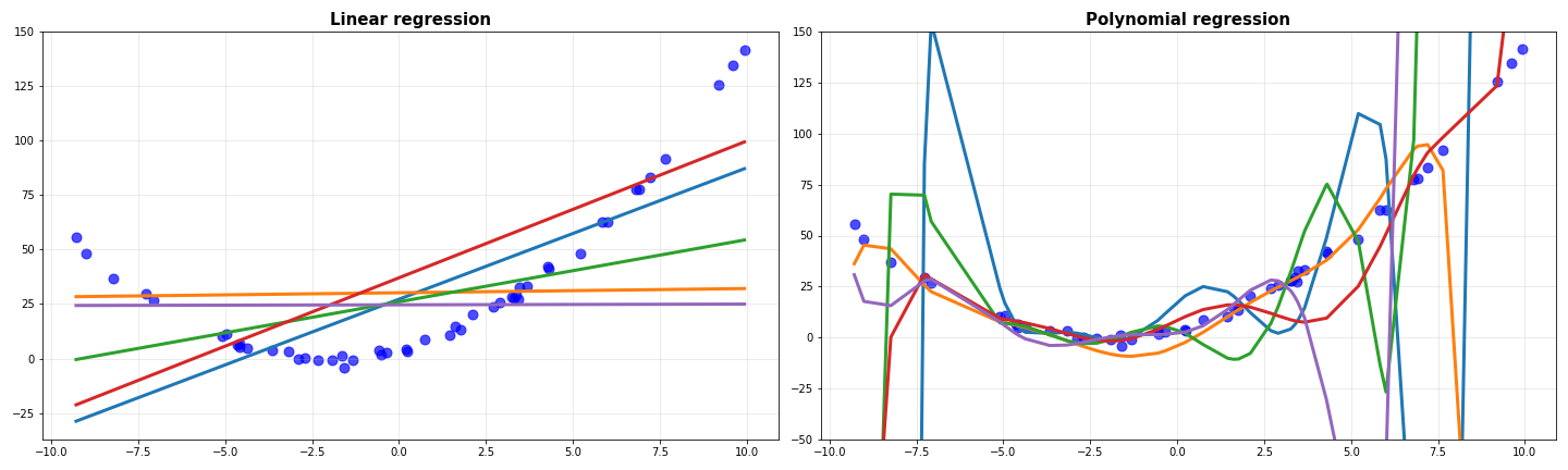
Notice how all the degree 1 models are quite similar to each other, while the degree 9 models are widely different. Before coming to the gist of this, I’ll do one more thing: I’ll average the predictions of all the models and plot them against the data.

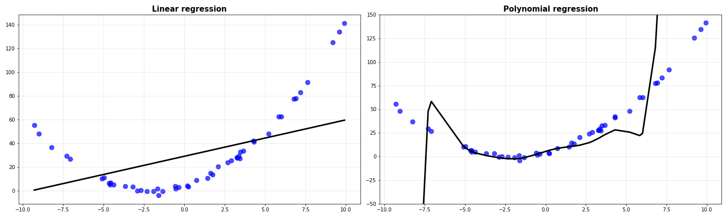
The average prediction of linear models is as bad as any of the others. However, the average for the degree 9 polynomial looks slightly better than all of them individually. Whatever we saw above is formalized using the ideas of bias and variance.

A model’s bias is defined as the average (expected) deviation between the model’s outputs and the targets.

The model’s variance is the expected squared difference between the model’s predictions and its long-run averaged predictions.

To make things more concrete, we can say that the linear model has high bias, since its predictions for most of the data points are far away from the targets. It also has low variance, since the model predicts more or less the same values even if the data changes. The complex degree 9 model has high variance, since it’s predictions vary wildly when the data changes. Plus, it has low bias since a good number of its predictions are close to the targets.

A model with high bias is very rigid; it doesn’t change much with data (low variance). A model with high variance is too flexible: it changes its configuration completely when the data changes. Below is a derivation to show how squared error loss gives way to bias and variance. Let $\hat{y}$ be the predicted function and $y$ be the targets. If the function that generated the data was $f(x)$, then the targets $y=f(x)+\epsilon$, where $\epsilon$ is noise. Noise is commonly characterized to a normal distribution whose mean is expected to be 0.

We can replace $y=f(x)+\epsilon$ as stated earlier, simplifying some terms.

Replacing it back, we get the following equation.

Now $f(x)$ is a deterministic function, which means it does not change with data. Thus, the expected value of this function (its average) is going to be the function itself ($\mathbb{E}\left[f(x)\right]=f(x)$).

We make a clever manipulation here by adding and subtracting the term $\left(\mathbb{E}\left[\hat{y}\right]\right)^{2}$ and rearranging the terms in the equation.

Recognize $\mathbb{E}\left[\hat{y}^{2}\right]-\left(\mathbb{E}\left[\hat{y}\right]\right)^{2} = \textrm{Var}\left[\hat{y}\right]$ and we have:

… which is actually:

Theoretically, the bias and variance of a model is expected to behave in the manner shown in the image below.

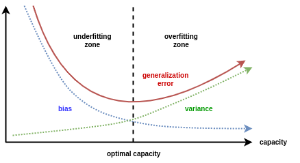
At the point where generalization error is minimum, both the bias and variance are quite small. This is the sweet spot we are looking for. This phenomenon, where reducing model bias results in increasing variance is known as the bias-variance tradeoff.

The same can be estimated by looking at the trends of training and validation errors as well. In general, we expect them to behave like this.

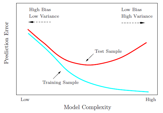
The validation error starts reducing as model complexity is increased, reaches a minimum around the right model and then starts increasing. When the model has high bias, both the training and validation errors are high. When it has high variance, the training error is quite low but the validation error is pretty high. The right model may also be considered as the one for which validation error minimizes.

Regularization: controlling variance

Let’s have a look at the regression coefficients of an overfit model. Actually, to get my point through, I’m going to show you the coefficients across 3 independent runs.

import numpy as np
from sklearn.linear_model import LinearRegression
from sklearn.preprocessing import PolynomialFeatures
from sklearn.linear_model import Lasso

coefs = []

for _ in range(3):
    
    # Train dataset 
    X_train = np.linspace(-1, 1, 100).reshape(-1, 1)
    y_train = (X_train + 10)**2 + np.random.normal(0, 1, 100).reshape(-1, 1)

    # Degree 9 model
    poly = PolynomialFeatures(degree=9)
    X_train_poly = poly.fit_transform(X_train)
    linreg = LinearRegression()
    linreg.fit(X_train_poly, y_train)
    coefs.append(linreg.coef_)

# Plot them 
fig = plt.figure(figsize=(20, 6))
for i, c in enumerate(coefs):
    ax = fig.add_subplot(1, len(coefs), i+1)
    pd.Series(c.reshape(-1,)).plot(kind='bar', color='b')
    ax.set_title("Run {}".format(i+1), fontweight='bold', fontsize=15)
    ax.grid(alpha=0.3)
    
plt.tight_layout()
plt.savefig("overfit_coefs.png")
plt.show()

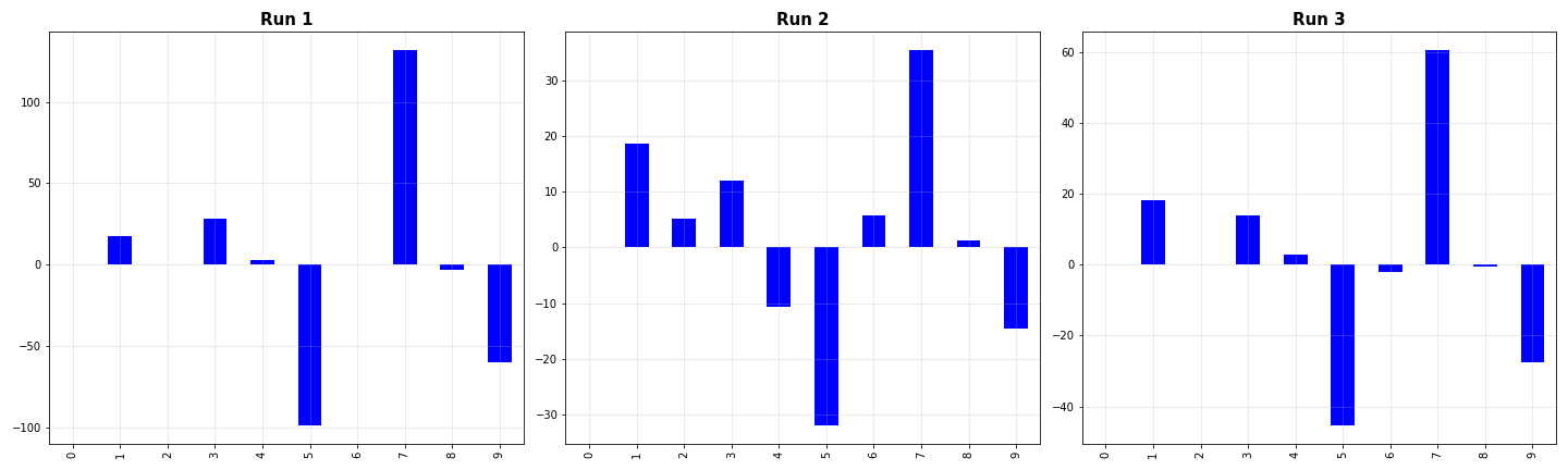
Even when the distribution of the data doesn’t change much, there is significant variation in the coefficients of the model. Especially, note how some coefficients are significantly larger than the others. This, in some way, explains the haphazard plots we saw earlier when fitting several degree 9 curves to quadratic data. The important question is: is there some way we can use such a complex model and and still get stable coefficients (reduce the variation)? Turns out there is! And if tuned properly, it can help curb the variation to a good extent. This process is called regularization.

The basic idea is that we penalize the model for making the parameters take extreme values (especially unusually high values). This is done by modifying the squared error function as follows.

Let’s take a closer look at how this works by choosing $g(\Theta)=\Theta^{T}\Theta$. This method is called $L_{2}$ regularization because here $g$ is the $L_{2}$ norm of the parameter vector. Regression performed with $L_{2}$ regularization is often called Ridge regression, which is also its name in scikit-learn.

The intuition for how this works is very obvious: if the magnitudes of any of the parameters becomes very large, the sum of squared coefficients will become large, increasing the loss overall. Thus, the model will be incentivized to reduce the magnitudes of large coefficients, while reducing the squared error itself.

Another popular choice for $g(\Theta)$ is the absolute values of the parameters, i.e. their $L_{1}$ norm. This method is often called LASSO Regression, where LASSO is an abbreviation for Least Absolute Shrinkage and Selection Operator.

LASSO is named that way because it has a special property, which can help us select important features by discarding the ones which have no impact on the targets.

Choice of $\lambda$

$\lambda$ is a hyperparameter which must be tuned to find the best performing model. Keeping very small values of $\lambda$ is similar to having no regularization, which means our model will retain the variance that it naturally has. Setting $\lambda$ to a very high value suppresses the weights excessively, which reduces the model’s variance so much that it reaches the underfitting region.

Let’s write some code and see how ridge regression and LASSO help us fit high dimensional models to data better. First, we need a mechanism to choose the right value of $\lambda$ (which is called alpha in scikit-learn functions). To do that, let’s perform a logspace search over $(-4, -1)$ to find the value of $\lambda$ for which the validation error is minimum (the domain $(-4, -1)$ was chosen after some trial and error). This means the values we will be searching in will be 10 logarithmically equally spaced values between $10^{-4}$ and $10^{-1}$.

import numpy as np
from sklearn.linear_model import LinearRegression, Ridge
from sklearn.preprocessing import PolynomialFeatures
from warnings import filterwarnings
filterwarnings(action='ignore')

np.random.seed(1)

# Train dataset 
X_train = np.linspace(-1, 1, 10).reshape(-1, 1)
y_train = (X_train + 0.5)**2 + np.random.normal(0, 0.1, 10).reshape(-1, 1)

# Validation dataset
X_val = np.sort(np.random.uniform(-1, 1, size=50)).reshape(-1, 1)
y_val = (X_val + 0.5)**2 + np.random.normal(0, 0.1, 50).reshape(-1, 1)

# Polynomial features
poly = PolynomialFeatures(degree=9)
X_train_poly = poly.fit_transform(X_train)
X_val_poly = poly.fit_transform(X_val)

# List to store MSE losses
losses = []

# List of regression parameters we will use
alphas = np.logspace(-4, -1, 10).tolist()

for lbd in alphas:    

    linreg = Ridge(alpha=lbd)
    linreg.fit(X_train_poly, y_train)
    linreg_preds = linreg.predict(X_val_poly)
    mse = mean_squared_error(y_val, linreg_preds)
    losses.append(mse)

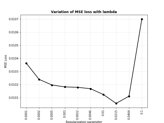
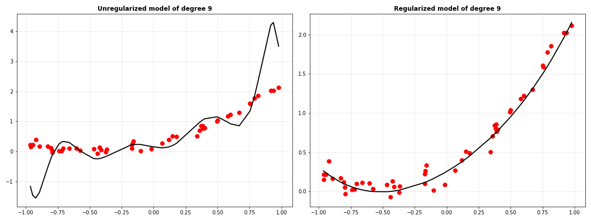
From the plot above, it seems that $\lambda=0.0215$ does best for our model. Let’s plot the fit curve when there is no regularization ($\lambda=0$) and with our best regularization parameters.

ridge = Ridge(alpha=0)
ridge.fit(X_train_poly, y_train)
no_reg_preds = ridge.predict(X_val_poly)

ridge = Ridge(alpha=0.0215)
ridge.fit(X_train_poly, y_train)
reg_preds = ridge.predict(X_val_poly)

fig = plt.figure(figsize=(16, 6))
ax1 = fig.add_subplot(121)
ax1.scatter(X_val, y_val, s=60, color='b')
ax1.plot(X_val, no_reg_preds, color='k', linewidth=2)
ax1.set_title("Unregularized model of degree 9", fontweight='bold')
ax1.grid(alpha=0.3)

ax2 = fig.add_subplot(122)
ax2.scatter(X_val, y_val, s=60, color='b')
ax2.plot(X_val, reg_preds, color='k', linewidth=2)
ax2.set_title("Regularized model of degree 9", fontweight='bold')
ax2.grid(alpha=0.3)

plt.tight_layout()
plt.savefig("noreg_vs_reg.png")
plt.show()

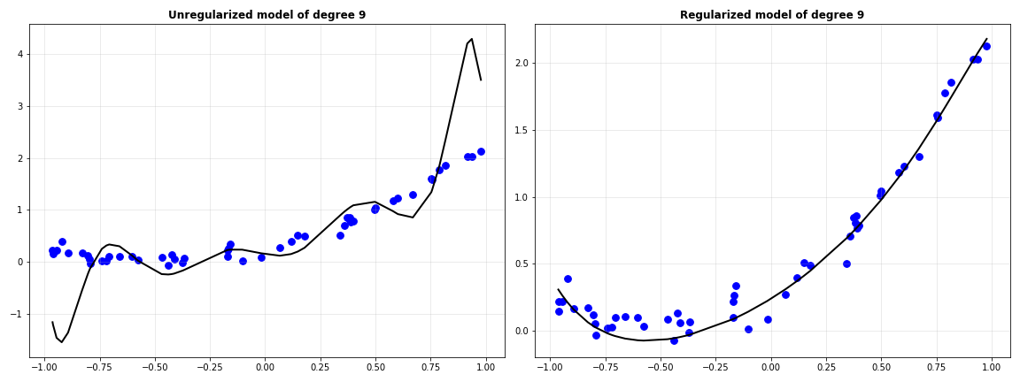
Clearly, regularization has made the model’s predictions much better. When the same experiment was performed with LASSO, this is the trend of MSE versus values of $\lambda$.

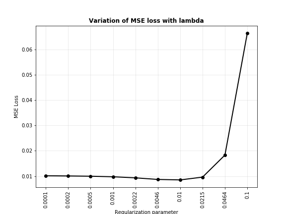
The best value for LASSO seems to be about $0.01$. This is how the regularized model looks against the unregularized model.

Not very different from ridge regression… for now. But there’s one major difference in how these two work, which makes LASSO useful for selecting important features for the model. Let’s look at the coefficients of the two regularized models with their best $\lambda$.

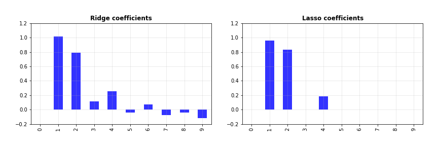
Let’s also print them out to see clearly what their values are.

print(ridge.coef_)

>>> [[ 0.          1.01955536  0.79269672  0.11758929  0.25340957 -0.03870505
       0.07197776 -0.07517875 -0.03745432 -0.11466282]]

print(lasso.coef_)

>>> [ 0.          0.95847276  0.83103968 -0.          0.1863634  -0.
      0.         -0.          0.         -0.        ]

Did you see that? For some of the features, ridge and LASSO have about the same coefficients. For others, while ridge gives them small but non-zero weights, LASSO drives their weights to zero. How is that useful? The coefficients, in a way, determine the contribution of their associated feature towards the target. If the coefficient of a feature is zero, that means regardless of what value it takes, it does not affect the target at all. This “un-usefulness” is identified by LASSO, and you can take advantage of this by discarding such features from the model. This helps reduce its complexity, which is beneficial.

Why does this happen anyway? Let’s start with the $L_{1}$ regularized loss function and study the resulting update rule. We’ll ignore the average constant because it has no bearing on the proof.

The gradient of the loss with respect to the parameters can be obtained as follows.

Now let’s say the model is described by the following equation. If we pre-multiply by $X^{T}$, we get the adjacent equation.

Now if we consider this model as a univariate system with $\Theta>0$, this will directly imply that $\boxed{X^{T}y>0}$. Going back to the update rule: if we start with $\lambda < X^{T}y$, we can increase it enough to drive $\Theta$ to zero. What happens if we increase it further? The sign of $\Theta$ changes and so does the update rule (remember that we had a modulus function there).

The new solution moves us away from the optimum, causing an increase in the loss (which the model does not want). So, it settles at $\Theta=0$. What about $L_{2}$ normed regularization?

Due to our assumption $\lambda > 0$, no value of $\lambda$ can make $\Theta=0$. Thus $L_{2}$ regularized regression will never give you zero coefficients. This argument can be extended to the case when $\Theta<0$. In multivariate systems there could be additional complexities where change in one feature’s coefficient affects that of another. However, it usually works out as it has done now in most situations.

Conculsion

That was a lot! From polynomial regression, to the problems with overly complex models, to regularization, we’ve covered a lot of ground in this post. Hopefully, you’re now in a position to choose the model with right complexity for your regression tasks. I’m going to leave regression here for now, and move to another (more popular) machine learning task: classification.