Accelerated and Stable Training

01 September 2020 - 16 mins read time
Tags: Calculus Linear Algebra Python

In the last post, I discussed how gradient descent and backpropagation can help tune the weights and biases of your nerual network so it can start performing better. However, from a practical viewpoint, this will lead to really unstable training and convergence might almost never happen. There are quite a few reasons for this.

1. Keeping the learning rate constant from start to end can be an issue. While high learning rates are needed when you are far from an optimum, you’ll want to take smaller steps when you’re close to one. We have done nothing to induce such behavior.
2. If the loss function is not smooth (will almost never be), local gradients might be significantly different from those in the neighborhood and the model’s performance will degrade with such an update. It’s like running down a hill studded with boulders. If you hit one, you’ll get confused and slow down.
3. Every neural network maps the input space to the output space using a complex function (possibly nonlinear) function. The outputs of the model follow a distribution generated by this mapped function. If the distribution of outputs experiences drastic changes throughout training, the model is not very confident about the mapped function. This is called Internal Covariant Shift; it makes convergence difficult.

Several techniques are incorporated with neural networks on top of backpropagation to make training much more stable and faster. In this post, I will discuss three of them: optimizers, learning rate scheduling and batch normalization.

Optimizers

Optimizers deal with two of the issues mentioned above: local gradients’ influence on training and constant learning rates. To begin, one very intuitive way of damping the effect of local gradients is to add some influence of past gradients or past weight updates to it. If you’re running down a hill and you see some rocks, you mustn’t let them distract you because in the past fews steps you’ve only been moving downwards and chances are you still have to do the same.

Generalized Delta Rule (Classical Momentum Method)

In this very basic upgrade, we include the previous weight update to the current one with some weightage, called the momentum. Momentum is one way of quantifying a system’s tendency to keep moving in the direction it has been going in the recent past.

In the expression above, $G_{w}(t)$ is the gradient of the loss function with respect to the weights, $\eta$ is the learning rate and $\alpha$ is the momentum. $\alpha$ is usually set to a value less than but reasonably close to $1$. If we unfold the equation above in time, we can obtain express the update solely in terms of gradients.

… and so on. In general, the update rule will look like the equation below.

Notice how the current gradient is given maximum weight and the previous gradients are given exponentially lower weight. Let’s understand why this kind of update should work, using our over-simplified loss function. We will focus on two different regions, marked $A$ and $B$.

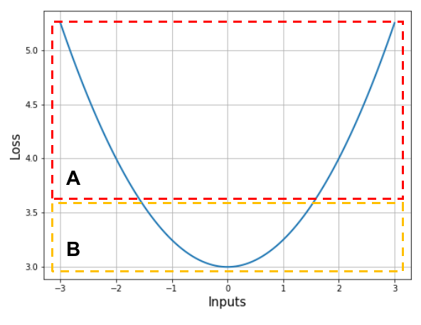
Region A. Notice how the loss function in region $A$ is almost a straight line, such that its slope isn’t changing much. Such regions are called low curvature regions. In this region, it is reasonable to assume that the gradient of the loss function will remain constant. In context of the equation above, the following can now be written.

The constant multiplied with $\eta$ will be bound by $\frac{1}{1-\alpha}$ (which is what the summation asymptotically converges to if it went on indefinitely). This means that the learning rate in low curvature regions will be constant, allowing us to traverse them quickly. Now let’s see what happens when we reach region $B$.

Region B. We enter region $B$ with a learning rate that’s pretty high. This causes the model to overshoot the optimum and reach the other side of the loss function, and the sign of the gradient changes. The gradient doesn’t change much and the overshoot happens again and the sign of the gradient changes as well. This is depicted in the diagram below.

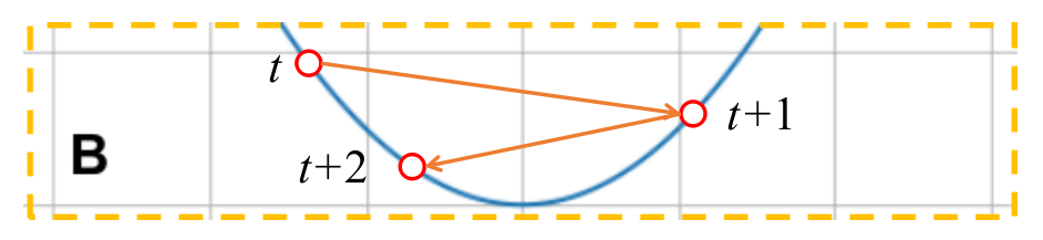
If we look at the parameter update at time $t$, the equation looks like this:

As we approach the minimum, the magnitudes of gradients keep getting smaller. That being said, the equation above indicates that a finite value is being subtracted from $G_{w}(t)$, reducing its effective magnitude. This subtracted quantity increases in magnitude with iterations, slowly reducing the amount of overshoot as time passes. After sufficiently long time, we will converge to the minimum.

Thus, the Generalized Delta Rule provides some improvement over vanilla gradient descent as far as dealing with local gradients is concerned. This optimizer is commonly available under the name Stochastic Gradient Descent (SGD) in popular deep learning libraries for Python like Tensorflow and Pytorch.

AdaGrad

AdaGrad attempts to change the effective magnitude of the learning directly by normalizing it with the overall magnitude of the total gradient so far. This is better understood by looking at its update equation, shown below.

Here, $\epsilon$ is a small number kept there to prevent math errors. As training progresses, more values keep getting added to $r_{w}(t)$ and the effective learning rate keeps getting smaller; assuming that the model is moving towards a minimum, this should be fine. Notice however that irrespective of where the model is in the parameters space, the learning rate will always reduce after every iteration. This may not be desirable in cases when the learning curve of the model is long, as the effective learning rate will become very small to result in any progress after some time. It is imperative that this optimizer is initialized with a sufficiently high learning rate and the magnitudes of gradients are kept under control, in case they should wander owing to the task the model is trying to learn.

RMSprop

RMSprop is a slightly modified version of AdaGrad, such that the LR (learning rate) shrinkage issue is controlled to some extent.

The learning rate is normalized majorly with the square root of the sum of squares of gradients from the last $L$ iterations: the RMS of the gradients from the last L iterations. We also provide some weight to gradients of this iteration. Since the average is performed over a fixed window, the magnitude of the learning rate might not reduce indefinitely, thus solving the issue we were facing in AdaGrad. $L$ is a hyperparameter to tune and $\rho$ is usually set to a value close to $1$, like $0.8$. It might be interesting to note that RMSprop has no official publication: it was proposed by Prof. Geoff Hinton in one of his lectures.

AdaDelta

AdaDelta was developed over an interesting observation: the units of the weight updates in AdaGrad do not match the units of the weights themselves (learning rate is dimensionless). Therefore, the authors made the following modification to the AdaGrad update, one of which we have already seen in RMSprop.

The denominator is similar to the one in RMSprop. The numerator is now a moving RMS over the last $L-1$ weight updates (since the current weight update is not known). This method is very popular due to the fact that one does not have to tune any learning rate parameter for it. Initially, the weight updates will be large in magnitude leading to large overall step size. As training progresses, the weight updates become smaller in magnitude and sparser, and the overall step size reduces. AdaDelta was developed by Matthew Zeiler when he was an intern at Google.

Adam

AdaGrad and AdaDelta are known as adaptive moments based methods, since they use the second moment of the gradients (root mean of gradients squared) to compute parameter updates. Adam, which literally stands for Adaptive Moments, keeps track of not only the second moment of gradients, but also the first moment (exponentially decaying average of the gradients themselves). These moments are maintained using the following equations.

Here, $q_{w}$ is the exponentially decaying average of gradients and $r_{w}$ is the same for the square of gradients. $q_{w}$ and $r_{w}$ are initialized to zeros. The authors noticed that this biased the averages towards zero, since $\beta_{1}$ and $\beta_{2}$ are typically set close to $1$ (thus giving large weight to prior values). To resolve this issue, the two terms are corrected of their bias this way:

Then, the parameter update is performed using the expression below.

The authors suggest setting $\beta_{1}=0.9$, $\beta_{2}=0.999$ and $\epsilon=10^{-8}$. It has been empirically shown that Adam outperforms the optimizers mentioned above in most cases. Therefore, it is the go-to optimizer for most tasks today. Several variations of Adam exist, sometimes customized for certain tasks. Some of them include AdaMax, Nadam and AdamW. You can read more about different kinds of optimizers in this blog post.

Learning rate scheduling

This method focuses more on modifying the learning rate itself. The optimizers attempt to tweak the effective step size of the model at every weight update. However, those containing $\eta$ do not change its value at all. By manually reducing the value of learning rate as training progresses, we can enforce small step sizes when we are close to an optimum. Several kinds of learning rate schedulers exist; quite often, they are manually designed for a particular task at hand since they have a fair bit of hyperparameter tuning to do. I’ve discussed few common tyeps of schedulers below.

Step LR scheduler

This method exponentially decays the learning rate by multiplying it with a constant $< 1$ every few iterations. By what factor the LR must be decayed and how often are hyperparameters to be chosen by the user.

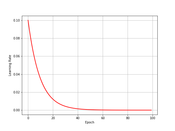
Careful tuning of $\gamma$ and the frequency of decay is necessary, since too quick a decay with slow down progress too much, and too slow a decay might not reduce LR sifficiently when close to an optimum.

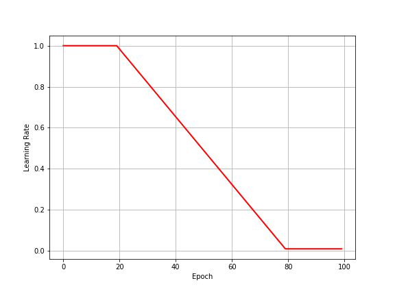
Linear or piecewise linear LR schedulers

Sometimes we want the learning rate to reduce linearly in some regions and stay constant in others. Below is an example of how you might want the learning rate to behave, with the code that generated it. If you are using a deep learning toolkit like PyTorch or Tensorflow, you may have to define the same in a class that inherits from their native schedulers.

def learning_rate(start, end, epoch, total_epochs):
    """
        In this scheduler, we want LR to stay constant for 
        the first 20% and last 20% epochs, and decay linearly
        elsewhere.
    """
    const_epochs = int(0.2 * total_epochs)
    decay_epochs = int(0.6 * total_epochs)
    
    if epoch < const_epochs:
        return start
    elif epoch < const_epochs + decay_epochs:
        return start - (start - end) * (epoch - const_epochs) / decay_epochs
    else:
        return end
    
etas = [learning_rate(1, 0.01, i+1, 100) for i in range(100)]    
    
plt.figure(figsize=(8, 6))
plt.plot(range(100), etas, linewidth=2, color="red")
plt.xlabel("Epoch")
plt.ylabel("Learning Rate")
plt.grid()
plt.show()

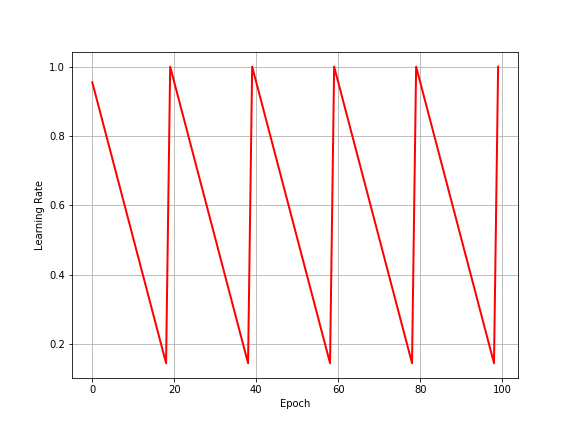
Cyclic LR schedulers

In some applications, you might want the learning rate to periodically attain a set of values. For example, let’s say your model trains on a set of data for some epochs, and then trains on another set of data for another few epochs. When the dataset is changes, you want the learning rate to get reinitialized to the starting value. You might do something like this:

def learning_rate(start, end, cycle_length, epoch, total_epochs):
    """
        In this scheduler, we want LR to decay from 1 to 0.1 every
        20 epochs then immediately be reset to 1.
    """
    return start - (start-end)*(epoch % cycle_length)/cycle_length
    
etas = [learning_rate(1, 0.1, 20, i+1, 100) for i in range(100)]    
    
plt.figure(figsize=(8, 6))
plt.plot(range(100), etas, linewidth=2, color="red")
plt.xlabel("Epoch")
plt.ylabel("Learning Rate")
plt.grid()
plt.savefig("cyclical_lr.png")
plt.show()

I don’t have much else to say about LR schedulers, apart from this. It is usually very helpful to manually design a scheduler that can help your model perform better for the specific task at hand.

Batch Normalization

Another aspect of ensuring smooth and productive training is to ensure that the parameters of the model do not sway too much across updates. Neural networks often fail to converge well is the variance of activations in several nodes keeps varying wildly. In totality, this means that the model’s confidence on the function it approximates is low and every other batch (or data point) is causing drastic changes in this function. This phenomenon is often called Internal Covariant Shift. One popular way to deal with this problem is batch normalization.

In batch normalization, the activations coming out of certain layers are normalized. This means, their distribution is coerced into a normal distribution, using some parameters which are learnt during training. That’s why, this process is also called Mean Variance Normalization. In general, the pipeline of batch normalization looks like the diagram below.

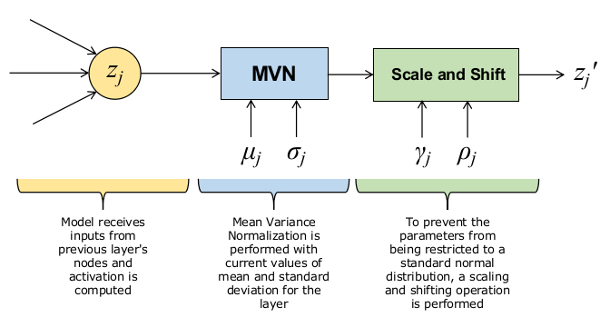
The update equations for these processes are as follows.

It is easy to compute the mean and variance of a batch of activations, done as follows. If the size of each mini-batch be $B$ and the batch normalization layer be present between the $L$ and $(L+1)^{th}$ layers of the model, then:

In its simplest form (shown above), the batch normalization layer learns 2 parameters: $\gamma_{j}$ and $\rho_{j}$. Batch normalization is used typically when the model is being trained in mini-batch mode, which means all parameter updates and loss calculations are averaged over small batches (subsets) of the entire dataset. The update equations for $\gamma_{j}$ and $\rho_{j}$ look like the ones given below. They can be derived by following the same procedure as followed for computing weight updates in backpropagation.

Let us quickly see how we can obtain the updates for the two parameters to be learnt: $\gamma_{j}$ and $\rho_{j}$. Assume the following network structure where the squares indicate the batch normalization layer. Inputs come in from the two nodes on the left end and outputs are collected on the right end.

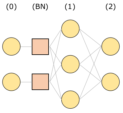
If you are unaware of the details of backpropagation, I recommend that you read my previous post, which will clarify my notation as well. No changes occur in that derivation for the output layer’s parameters, so let’s target the batch normalization layer directly.

$\gamma_{j}$ affects all $z_{l}^{(1)}$, so we have to retain the summation for further calculation.

In the above equation, note that $\gamma_{j}$ will only affect the output of the very node from the input layer that it is connected to: $z_{j}’^{(0)}$.

We know the expression for $z_{j}’^{(0)}$ as output from the batch normalization layer. Let’s isolate that partial derivative and simplify its expression.

That done, we can put everything together to compute the final gradient of the loss function with respect to $\gamma_{j}$. Also notice that some rearrangement and grouping of terms (as shown below) will reveal that this equation can be written in terms of local gradients of the layers.

This gradient can now be passed on to an optimizer which will perform suitable updates to the parameter. In a similar fashion, we can compute the update for $\rho_{j}$ and end up with this expression.

Layer Normalization

In some applications, we would want the activations coming out of a certain layer to follow a normal distribution for every example in the batch, regardless of whether the model is being trained in mini-batch mode or not. This is done through layer normalization, which is just mean variance normalization for each example.

Conclusion

In this article, I went over some important tools that are ubiquitously used with neural networks to provide stable and quick convergence. A lot of research is happening in this area, with several variations of the above technique producing small and large improvements in model training. Many learners often use these in their data science pipelines with less understanding of the several options they have and how they impact their model. Hopefully, this content has helped you become more aware of the underlying principles behind accelerated and stable learning.